How to migrate to the new Boulder Opal package

In this user guide we demonstrate the key points on how you can quickly and efficiently migrate your pre-existing Boulder Opal code from using the qctrl package to the new Boulder Opal client package boulderopal. Migrating to the new Boulder Opal client package comes with many advantages meant to accelerate development pace and help you get the most out of your Boulder Opal subscription.

These benefits include:

A simplified interface. The new boulderopal client supports more natural object types (like NumPy arrays) and simpler syntax (for instance, requiring less code), especially for closed-loop optimization and noise reconstruction.
Improved error handling. We are now able to detect errors on the client side that we could not previously with the legacy qctrl client, so the error and warnings are surfaced earlier to you, can be more informative, and ultimately save you compute time.

Installing the Boulder Opal Python client

You can install the Boulder Opal Python client using pip on the command line.

pip install boulder-opal

Overview of general interface changes

The motivation behind some of the changes outlined below was to make Boulder Opal accessible using a more Pythonic paradigm. As you will see, the boulderopal package provides a more intuitive and simple interface for accessing Boulder Opal's functionality. To achieve this, several substantial changes were made, as follows.

The `Qctrl` object

The new boulderopal package no longer features a Qctrl object. You can import it as a regular Python package and use its functions without reference to a session object.

import boulderopal as bo

Authentication

The first time you call a function from the boulderopal package that involves the cloud, your Boulder Opal session will be authenticated. This may mean that a browser window pops up asking you to log into the account associated with your Boulder Opal subscription, or if you've signed-in recently, it will automatically authenticate from a temporary token which gets saved on your local machine.

Organizations

If you're in more than one organization, you need to select which organization's resources to use when running calculations on the cloud. This can be done with boulderopal.cloud.set_organization, with your organization's slug. To find your organization's slug, view your plan details in the Boulder Opal web app.

bo.cloud.set_organization("your-organization-slug")

Function input/output changes

You don't need to pass the parameters to functions and class constructors as keyword arguments (as you needed to in the legacy client).

The functions in the Boulder Opal client return a dictionary, instead of a custom Boulder Opal object. This was done to make results more intuitive and easy to work with. For example, to access the output of a graph calculation, use result["output"] rather than the previous result.output.

Graph calculations export PWC nodes as a dictionary with "durations", "values", and "time_dimension" keys (rather than nested lists of "duration"/"value" dictionaries as in the legacy client). The "durations" and "values" of the piecewise-constant function are represented as NumPy arrays, and the "time_dimension" integer indicates the dimension of the values corresponding to time.

Functionality in the new client

Graph-based functionality

Instantiating a graph

You can instantiate a graph by calling its constructor at boulderopal.Graph.

graph = bo.Graph()

Graph operations

Some graph operations have been moved.

A new graph.random namespace contains graph operations with random behavior, such as graph.random.uniform.
A new graph.ions namespace contains graph operations dealing with trapped ion systems, such as graph.ions.ms_phases.
The legacy graph utils namespace has been removed; its operations can be directly accessed from the graph object via graph.complex_optimizable_pwc_signal, graph.real_optimizable_pwc_signal, and graph.filter_and_resample_pwc.

Note that graph.filter_and_resample_pwc now accepts a kernel rather than a cutoff_frequency, so you can now use this node with both a graph.gaussian_convolution_kernel or a graph.sinc_convolution_kernel.

Graph calculations

To execute graphs use boulderopal.execute_graph. Its inputs work very similarly to the legacy function qctrl.functions.calculate_graph.

import numpy as np

graph = bo.Graph()

amplitude = np.pi * 1e5  # rad/s
duration = 5e-6  # s

pi_pulse = graph.constant_pwc(amplitude, duration)
infidelity = graph.infidelity_pwc(
    hamiltonian=pi_pulse * graph.pauli_matrix("X"),
    target=graph.target(graph.pauli_matrix("X")),
    name="infidelity",
)

result = bo.execute_graph(graph, "infidelity")
print(f"π-pulse infidelity: {result['output']['infidelity']['value']:.3e}")

Your task (action_id="1812227") is queued.
Your task (action_id="1812227") has started.
Your task (action_id="1812227") has completed.
π-pulse infidelity: 4.441e-16

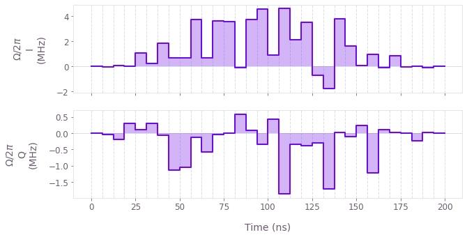
Graph optimization

To optimize graphs use boulderopal.run_optimization. Its inputs work very similarly to the legacy function qctrl.functions.calculate_optimization.

import qctrlvisualizer as qv

# Define physical constraints.
omega_max = 2 * np.pi * 6e6  # Hz
delta_max = 2 * np.pi * 3e6  # Hz
segment_count = 32
duration = 200e-9  # s

graph = bo.Graph()

# Create optimizable signal.
envelope = graph.signals.cosine_pulse_pwc(
    duration=duration, segment_count=segment_count, amplitude=1.0
)
omega = envelope * graph.complex_optimizable_pwc_signal(
    segment_count=segment_count, maximum=omega_max, duration=duration
)
omega.name = r"$\Omega$"

# Create Hamiltonian and define infidelity.
hamiltonian = graph.hermitian_part(omega * graph.pauli_matrix("X"))
infidelity = graph.infidelity_pwc(
    hamiltonian=hamiltonian,
    target=graph.target(operator=graph.pauli_matrix("X")),
    name="infidelity",
)

# Run the optimization.
result = bo.run_optimization(
    graph=graph,
    cost_node_name="infidelity",
    output_node_names=r"$\Omega$",
    optimization_count=4,
)

print(f"Optimized infidelity: {result['cost']:.3e}")

qv.plot_controls(result["output"], polar=False)

Your task (action_id="1812228") has started.
Your task (action_id="1812228") has completed.
Optimized infidelity: 1.110e-14

png-1

You can similarly use the other graph-based optimizers with boulderopal.run_stochastic_optimization or boulderopal.run_gradient_free_optimization.

Closed-loop optimization

The functionality to perform closed-loop optimization is in the boulderopal.closed_loop module, featuring two main functions to perform closed-loop optimizations: boulderopal.closed_loop.optimize and boulderopal.closed_loop.step.

boulderopal.closed_loop.optimize sets up a closed-loop optimization loop and runs it until a stopping criterion is met. It works very similarly to the legacy client's toolkit function qctrl.closed_loop.optimize, although there are a few small differences. See the function's reference page or this user guide for more information.

In those cases where boulderopal.closed_loop.optimize is not flexible enough, you can set up your own loop using boulderopal.closed_loop.step, which performs a single closed-loop optimization step. This works very similarly to the legacy function qctrl.functions.calculate_closed_loop_optimization_step, although we have simplified its inputs to make them more intuitive. See the function's reference page or this user guide for more information.

Noise reconstruction

The noise reconstruction functionality has been rebuilt from the ground up to have more natural inputs. Please look at the reference documentation and this user guide for more details.

Pulse library

The (non-graph-based) pulse library (originally in qctrl.signals) can be accessed through the boulderopal.signals namespace.

cosine_pulse = bo.signals.cosine_pulse(duration=10e-9, amplitude=5e6, drag=0.1)
cosine_pulse.export_with_time_step(1e-9)

array([ 122358.70926212-4.85402760e+13j, 1030536.86926882-1.27080092e+14j,
       2500000.        -1.57079633e+14j, 3969463.13073118-1.27080092e+14j,
       4877641.29073788-4.85402760e+13j, 4877641.29073788+4.85402760e+13j,
       3969463.13073118+1.27080092e+14j, 2500000.        +1.57079633e+14j,
       1030536.86926882+1.27080092e+14j,  122358.70926212+4.85402760e+13j])

Ions and superconducting toolkits

The system-specific toolkits (originally in qctrl.ions and qctrl.superconducting) can be found in the boulderopal.ions and boulderopal.superconducting modules.

The functionality remains the same, but some of the function signatures have changed slightly. For example, the parameter order has been tweaked, and the returned object is a direct graph calculation object (so the keys and contents of the resulting dictionary are different). See the reference documentation for the ions and superconducting modules for more information.

Managing calculations

Parallel calculations

Depending on your Boulder Opal plan and the number of available machines in your environment, you can run calculations in parallel. You can preprovision your environment before submitting your tasks by bringing machines online using boulderopal.cloud.request_machines.

You can also group multiple calculations and queue them together with boulderopal.cloud.group_requests, like with the legacy function qctrl.parallel. The results of the grouped calculations will be returned at the same time.

For more information, you can read the Computational resources in Boulder Opal topic or consult the reference documentation.

Retrieving results

You can retrieve results from previous calculations using boulderopal.cloud.get_result. This is equivalent to the legacy qctrl.get_result.

Removed functionality

Simulation functions

The legacy simulation functions (qctrl.functions.calculate_colored_noise_simulation, qctrl.functions.calculate_coherent_simulation, and qctrl.functions.calculate_quasi_static_scan) have been replaced by graph calculations. Please use a graph calculation instead. For more information, some relevant user guides about representing quantum systems in graphs, performing noiseless simulations, performing quasi-static scans, and performing simulations involving noise.

Filter functions

The legacy function to calculate filter functions (qctrl.functions.calculate_filter_function) has also been replaced by graph calculations in the new client, using the graph.filter_function operation. Calculating them in a graph is more flexible and faster. You can find more information in this user guide.

Cross-entropy closed-loop optimizer

The cross-entropy method is not available in the new client. You can use any of the other closed-loop optimizers as they're bound to return better results.

Reinforcement learning

The reinforcement learning features from the Q-CTRL Python package have not been migrated to the new client yet.