How to calculate system dynamics for arbitrary Mølmer–Sørensen gates

Boulder Opal enables you to optimize, explore and validate the dynamics induced by Mølmer–Sørensen-type operations. In this notebook, we begin with an optimized control and show how to obtain the evolution dynamics of the entangling phase and the motional trajectories in phase space, using convenience functions designed for trapped-ion experiments.

You can learn how to optimize error-robust Mølmer–Sørensen gates for trapped ions in our user guide, or perform complex operations by designing robust, configurable, parallel gates for large trapped-ion arrays using our application note.

Summary workflow

1. Define and calculate ion properties

To find optimized drives, you first need to know the physical properties of the ions, namely the Lamb–Dicke parameters and mode frequencies. You can calculate these values using the function boulderopal.ions.obtain_ion_chain_properties by providing basic parameters of your ion trap, specifically the mass of the ions, center of mass frequencies, and laser wave numbers along different axes. The function returns the Lamb–Dicke parameters and relative detunings as 3D and 2D arrays, respectively, which will be used in the phase and displacement calculations.

2. Calculate motional displacement trajectories and phase dynamics

Given the controls, you can obtain the gate dynamics. In particular, you can visualize the trajectory of the center of a coherent state in (rotating) optical phase space for each mode. The closure of these trajectories is a necessary condition for an effective operation. You can also obtain the phase accumulation during the gate operation for each pair of ions, and the target phases should be achieved at the end of a successful operation.

You can utilize our flexible boulderopal.execute_graph function to track how displacements and phases change during the gate operational time. Within a graph, you can include the graph.ions.ms_phases and graph.ions.ms_displacements operations that take the control drives and ion properties as inputs. You can simply provide the sample_times parameter with your desired time sampling for the evolution, and use boulderopal.execute_graph to return the dynamics.

Note that the results of the graph.ions.ms_displacements function describe contributions to each mode from each ion. To get the overall displacement for each mode, you need to sum over the ion dimension (see the notes of graph.ions.ms_displacements for details).

Example: GHZ state on a chain of three ions

In this example we consider a chain of three ions (${}^{171}{\rm Yb}^{+}$), and the goal is to examine the dynamics induced by drives that have been optimized to generate a relative phase of $\pi/4$ between each ion pair. Note that you can perform $X_{\pi/2}$ rotations for all ions after applying the optimal drives to create the GHZ state, as shown in Kim et al. (2009).

Define and calculate ion properties

We begin by calculating ion properties based on inputs relevant to the system under examination.

import jsonpickle
import matplotlib.pyplot as plt
import numpy as np
import qctrlvisualizer as qv
import boulderopal as bo

plt.style.use(qv.get_qctrl_style())


def load_variable(file_name):
    """
    Load a variable from a file encoded with jsonpickle.
    """
    with open(file_name, "r+") as file:
        return jsonpickle.decode(file.read())


data_folder = "./resources/"

# Specify ion trap parameters.
ion_count = 3
atomic_mass = 171
center_of_mass_frequencies = [1.6e6, 1.5e6, 0.3e6]

# Define laser characteristics.
wavevector = [1.8e7, 1.8e7, 0]
laser_detuning = 1.6047e6
maximum_rabi_rate = 2 * np.pi * 100e3

# Calculate the ion chain properties:
# Lamb–Dicke parameters as an array of shape [<axis>, <collective_mode>, <ion>],
# Relative detunings as an array of shape [<axis>, <collective_mode>].
ion_chain_properties = bo.ions.obtain_ion_chain_properties(
    atomic_mass=atomic_mass,
    ion_count=ion_count,
    center_of_mass_frequencies=center_of_mass_frequencies,
    wavevector=wavevector,
    laser_detuning=laser_detuning,
)
lamb_dicke_parameters = ion_chain_properties["lamb_dicke_parameters"]
relative_detunings = ion_chain_properties["relative_detunings"]

Your task (action_id="1828012") has completed.

Import optimized drives

Next, we import the optimized drive data. The drives have been optimized to generate $\pi/4$ relative phase between each ion pair in a chain of three ions.

drive_data = load_variable(data_folder + "optimized_drives")
qv.plot_controls(drive_data)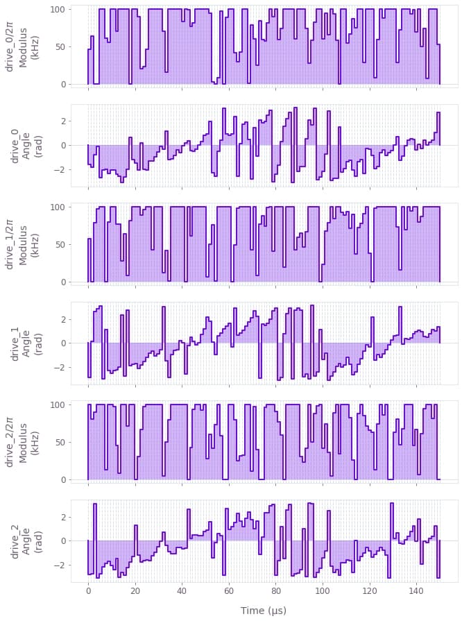

The drives are displayed above, where an individual drive, drive_j, is applied to each ion j with optimized modulation in the modulus and phase (or angle).

Calculate relative phase and motional displacement dynamics

Here we apply our boulderopal.execute_graph function to obtain the motional displacement trajectories and the relative phases for the duration of the given drives, with specified sample_times.

drive_names = list(drive_data.keys())
duration = np.sum(drive_data[drive_names[0]]["durations"])
sample_times = np.linspace(0, duration, 100)

graph = bo.Graph()

# Collect optimized drives.
drives = [graph.pwc(**drive_data[name]) for name in drive_names]

# Calculate phases and displacements.
ms_phases = graph.ions.ms_phases(
    drives=drives,
    lamb_dicke_parameters=lamb_dicke_parameters,
    relative_detunings=relative_detunings,
    sample_times=sample_times,
    name="phases",
)
ms_displacements = graph.ions.ms_displacements(
    drives=drives,
    lamb_dicke_parameters=lamb_dicke_parameters,
    relative_detunings=relative_detunings,
    sample_times=sample_times,
    name="displacements",
)

# Execute the graph.
result = bo.execute_graph(graph=graph, output_node_names=["phases", "displacements"])

Your task (action_id="1828013") has started.
Your task (action_id="1828013") has completed.

Now we can calculate the contribution of each ion to the mode displacements, and plot the mode displacement trajectories.

trajectories = np.sum(result["output"]["displacements"]["value"], axis=3)
plot_range = 1.05 * np.max(np.abs(trajectories))

fig, axs = plt.subplots(1, 2, figsize=(10, 5))
fig.suptitle("Phase space trajectories", y=1.1)

for k in range(2):
    for mode in range(ion_count):
        axs[k].plot(
            np.real(trajectories[:, k, mode]),
            np.imag(trajectories[:, k, mode]),
            label=f"mode {mode % 3}",
        )
        axs[k].plot(
            np.real(trajectories[-1, k, mode]),
            np.imag(trajectories[-1, k, mode]),
            "kx",
            markersize=15,
        )

    axs[k].set_xlim(-plot_range, plot_range)
    axs[k].set_ylim(-plot_range, plot_range)
    axs[k].set_aspect("equal")
    axs[k].set_xlabel("q")

axs[0].set_title("$x$-axis")
axs[0].set_ylabel("p")
axs[1].set_title("$y$-axis")
axs[1].yaxis.set_ticklabels([])

hs, ls = axs[0].get_legend_handles_labels()
fig.legend(handles=hs, labels=ls, loc="center", bbox_to_anchor=(0.5, 1), ncol=ion_count)

plt.tight_layout()
plt.show()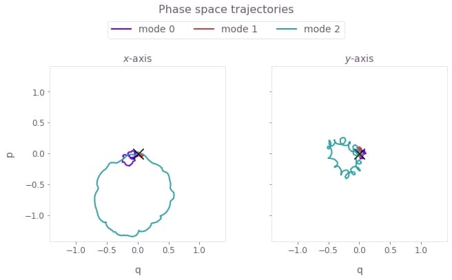

Here, $q \equiv q_m = (a_m^\dagger + a_m)/\sqrt{2}$ and $p \equiv p_m = i (a_m^\dagger - a_m)/\sqrt{2}$ are the dimensionless quadratures for each mode $m$ and its corresponding annihilation operator $a_m$. The black cross marks the final displacement for each mode. These are overlapping at zero, indicating no residual state-motional entanglement and no motional heating caused by the operations. The z-axis modes are not addressed, and thus have no excursions in phase space.

Next we obtain and visualize the relative phase dynamics for each pair of ions.

# Recall that the phases are stored as a strictly lower triangular matrix.
# See the notes of the ms_phases graph operation.
phases = result["output"]["phases"]["value"]

# Plot phase dynamics.
plt.plot([0, sample_times[-1] * 1e3], [np.pi / 4, np.pi / 4], "k--")
for ion_1 in range(3):
    for ion_2 in range(ion_1):
        plt.plot(sample_times * 1e3, phases[:, ion_1, ion_2], label=f"{ion_2, ion_1}")

plt.legend(title="Ion pair")
plt.xlabel("Time (ms)")
plt.ylabel("Relative phase")
plt.show()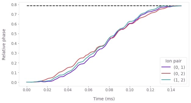

The figure shows the dynamics of the relative phase between the three pairs of ions, over the duration of the gate. Under the optimized controls, the relative phases evolve from 0 to the target phase of $\pi/4$ at the end of the operation (marked by the horizontal dashed line). This indicates a successful operation.