How to integrate Boulder Opal with QUA from Quantum Machines

Boulder Opal enables you to design and benchmark noise-robust pulses, as well as characterize and tune up your quantum hardware with ease. This process becomes even simpler and more powerful when software and hardware are seamlessly integrated.

In this notebook we show how to interface Boulder Opal with QUA, a programming language developed by Quantum Machines that provides pulse-level control of their Operator-X (OPX) quantum devices. Using the qctrl-qua package, we show how to convert a pulse into an OPX-compatible format and to quickly generate the configurations required for executing experiments.

Summary workflow

1. Define the QUA configuration

Before you can run any experiment, you first need to provide QUA with a thorough description of the quantum device. This "QUA configuration" is a Python dictionary containing instructions for configuring the QM hardware. It typically contains line calibrations, drive frequencies and pulse shapes for quantum gates. For more details, see the QUA examples in the QUA reference documentation.

2. Convert Q-CTRL pulses to QUA-compatible pulses

Now that you have a pre-existing QUA configuration, qm_config, you can take the Q-CTRL optimized pulse and add it to your QUA pulse library. For convenience, we will use add_pulse_to_config function from the qctrlqua package. This function accepts a pulse sampled at 1ns intervals and returns an appropriately-formatted Python dictionary that you can feed into the OPX. For more details, see the qctrl-qua reference documentation.

Example: Export a Gaussian pulse to a QUA backend

In the following example, we will import a pulse from the libraries of signals for Boulder Opal, as described in the reference documentation, and convert it into a QUA-compatible format. Although we use the example of a Gaussian pulse but the exact shape of the pulse we import is not important to illustrate the conversion.

Afterwards, the pulse is resampled to match the 1ns resolution of the hardware.

import numpy as np
import matplotlib.pyplot as plt
import qctrlvisualizer as qv
import boulderopal as bo
import qctrlqua

plt.style.use(qv.get_qctrl_style())

# Create Gaussian pulse.
total_rotation = np.pi  # π pulse
max_rabi_rate = 2 * np.pi * 50e6  # rad/s
duration = total_rotation * 10 / max_rabi_rate / np.sqrt(2 * np.pi)

control_pulse = bo.signals.gaussian_pulse(
    amplitude=max_rabi_rate, drag=0.1 * duration, duration=duration
)

# Resample the pulse to match the hardware time resolution.
dt = 1e-9  # s
resampled = control_pulse.export_with_time_step(dt)

# Map the optimal pulse into input amplitudes for the hardware.
rabi_rate = 2 * np.pi * 300e6  # rad/s
qctrl_i = np.real(resampled) / rabi_rate
qctrl_q = np.imag(resampled) / rabi_rate

# Plot resulting arrays.
plt.plot(qctrl_i, label="$I$")
plt.plot(qctrl_q, label="$Q$")
plt.xlabel("Time (ns)")
plt.ylabel("Voltage (V)")
plt.legend()
plt.show()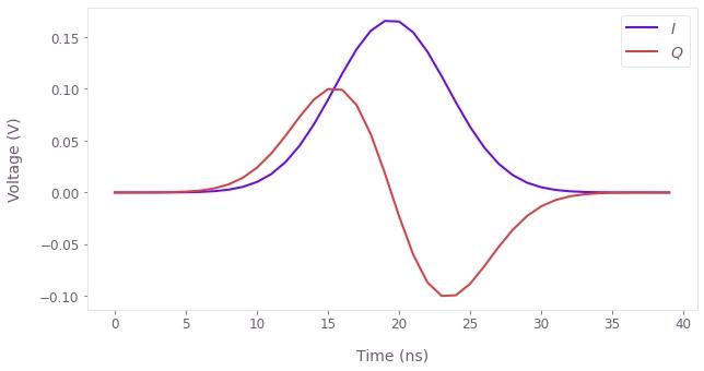

qm_config = {}
# Add the Q-CTRL robust pulse to the QUA configuration.
pulse_name = "Q-CTRL"
channel_name = "drive_channel"  # drive channel name in qm_config
qm_config = qctrlqua.add_pulse_to_config(
    pulse_name, channel_name, qctrl_i, qctrl_q, qm_config
)

# Use the updated qm_config dictionary to run QUA on the hardware.