How to automate complex calibration tasks with Boulder Opal
Automate your calibration workflows with the Q-CTRL Experiment Scheduler
The Q-CTRL Experiment Scheduler package for Boulder Opal allows you to automate the workflow of complex calibration procedures. The scheduler will take into account the dependency between different parts of the calibration, the status of each of this parts, and the parameters that you are most interested in the calibration. With this information, it will determine the sequence that the calibrations have to be executed and run them for you.
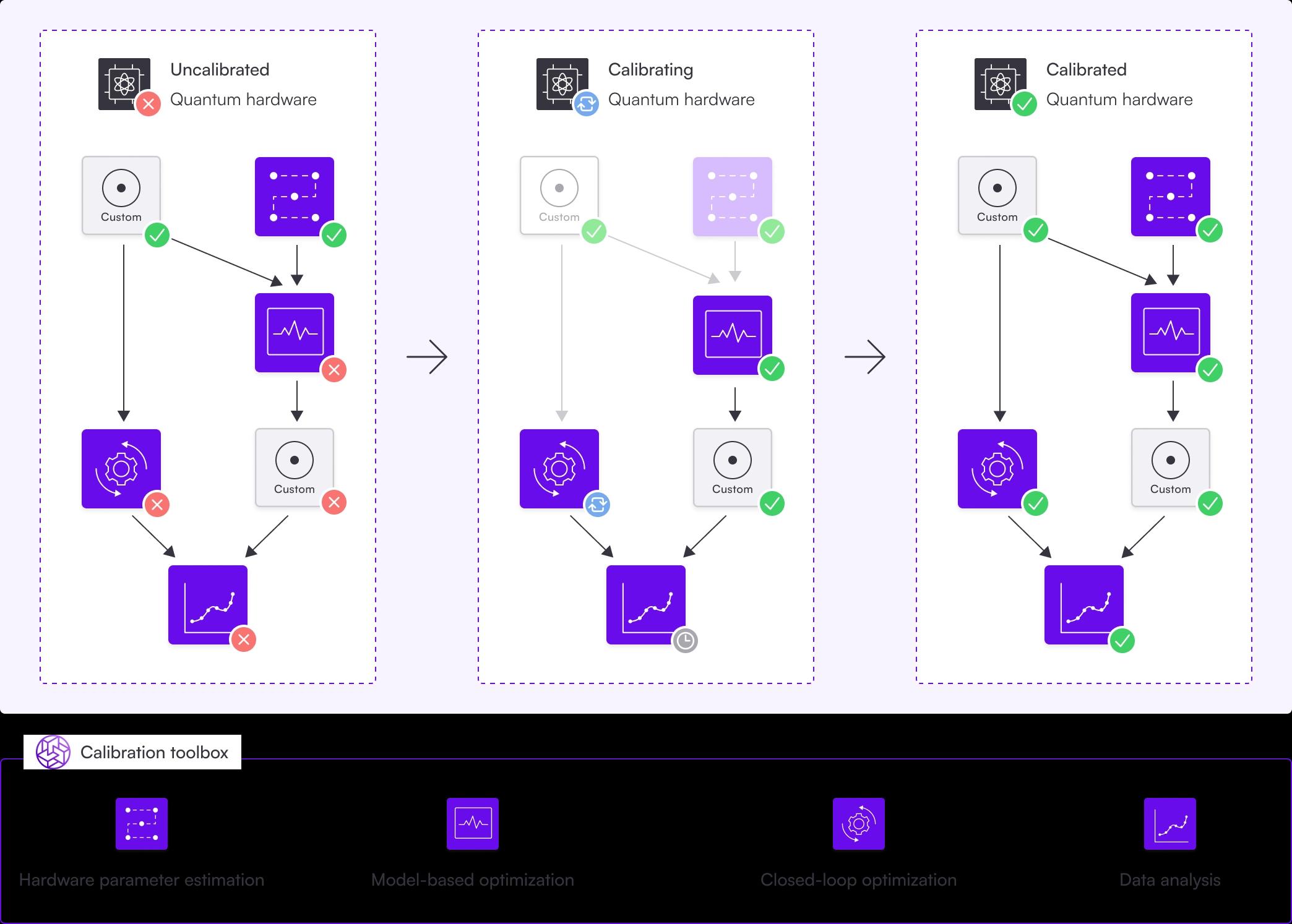
The calibration procedure is represented by a directed acyclic graph, where each node represents a step in the calibration. You can use many of Boulder Opal's features in these steps, like hardware parameter estimation, model-based optimization, or closed-loop optimization.
The dependency between nodes is represented by arrows, symbolizing the graph's edges. A node's dependents are those nodes with arrows pointing towards it: before a node can be calibrated, all of its dependents need to be calibrated first. For example, a dependency between two nodes could be the rough calibration of a parameter followed by a finer calibration using the value obtained in the rough calibration.
A graph traversal algorithm is used to find the optimal sequence of calibrations for the uncalibrated nodes, avoiding unnecessary calibrations of nodes already calibrated. Some algorithms (like Optimus) use additional information, like an automatic timeout duration indicating that the node has to be recalibrated. After the algorithm has traversed the graph, depending on the graph's purpose, the whole experiment has successfully run or the system is calibrated and ready to be used.
The Q-CTRL Experiment Scheduler is currently in alpha phase of development. Breaking changes may be introduced.
You can install the Q-CTRL Experiment Scheduler using pip on the command line.
pip install qctrl-experiment-schedulerThis user guide shows an example of how to run a simple amplitude calibration task using a predefined calibration graph. After that, it also shows how to customize the calibration procedure with your own extra steps.
Summary workflow
1. Define your calibration graph
The Q-CTRL Experiment Scheduler represents a complex calibration in the form of an directed acyclic graph, where each node represents a step of the calibration. Each node contains the routines to run a certain calibration, and the subsequent data analysis required to update the associated parameters, which are also stored in the calibration graph. The edges of the graph are the dependencies of a calibration: if an edge goes from node "A" to node "B", then it means calibration "B" requires "A" to be calibrated before the calibration "B" is executed. In this sense, the direction of the arrows reflects the temporal order in which the calibrations are performed.
The Q-CTRL Experiment Scheduler comes with predefined calibration graphs in the qctrlexperimentscheduler.predefined module.
These calibration graphs represent common calibration routines, and may be run in different architectures, or in a simulated environment using Boulder Opal.
To select which environment to run them, pass one of the predefined backends to the predefined graph.
You can also start a new calibration graph from scratch by instantiating a new CalibrationGraph object.
2. Add any further customizations
The Q-CTRL Experiment Scheduler gives the liberty for you to add more nodes to the calibration graphs, even the predefined ones.
To add more nodes to them, use the create_node method of the CalibrationGraph object.
Pass to the node a calibration_function that performs its calibration and updates any parameters accordingly.
This function accepts the CalibrationGraph as an input, and returns a CalibrationStatus indicating whether the calibration has succeeded (CalibrationStatus.PASS) or failed (CalibrationStatus.FAIL).
If the new node assumes that certain parts have already been calibrated by the time the calibration is run, add the required nodes to the list dependencies when calling create_node.
By default, it will be assumed that the node has no dependencies.
You can also add extra calibration parameters via the create_variable method.
3. Execute the calibrations in the graph
After your graph is built, it is time to run the calibration.
You can display the graph structure by using the method visualize().
From the graph, select a final node that will perform the most refined calibrations of all the variables you are interested, while also calibrating all the other variables on the way. This will be a node that is not a dependency of any other nodes.
After you've chosen the right node, call the method execute(), passing the node name a parameter.
The Q-CTRL Experiment Scheduler will then run all the calibrations necessary to find the right values of the parameters calibrated by that node.
After they are all run, you can retrieve the values of the calibrated parameters with get_variable().
Example: Running a predefined graph for amplitude calibration
The Q-CTRL Experiment Scheduler comes with predefined graphs to help you perform common calibration tasks.
The example below shows how a user can import one of these predefined graphs for a simple calibration of amplitudes of Gaussian $\pi$ and $\pi/2$ pulses. The backend selected is a simple simulator with high dephasing noise.
The graph contains three nodes, one for coarse calibration of the two amplitudes, and one for the fine calibration of each of the amplitudes, respectively. The only two parameters optimized are the amplitudes of the two gates.
The code example shows how to import a predefined graph, plug it to a backend, and then run the calibrations. It also shows how to visualize the graph.
import numpy as np
import matplotlib.pyplot as plt
import qctrlvisualizer as qv
import boulderopal as bo
import qctrlexperimentscheduler as es
from qctrlexperimentscheduler.predefined import (
    SimulationAmplitudeCalibrationBackend,
    create_amplitude_calibration_graph,
)

plt.style.use(qv.get_qctrl_style())

# Mute messages from Boulder Opal calls.
bo.cloud.set_verbosity("QUIET")
# Define a backend, that is, a way for the graph to communicate with
# the hardware that performs the calibrations. In this case, instead of
# hardware we define a simulation with high noise.
backend = SimulationAmplitudeCalibrationBackend(
maximum_rabi_rate=5e7, pulse_duration=320e-9, time_step=0.25e-9, dephasing_noise=4e5
)
# Create an instance of the predefined calibration graph.
calibration_graph = create_amplitude_calibration_graph(backend=backend)
# Visualize the graph.
calibration_graph.visualize()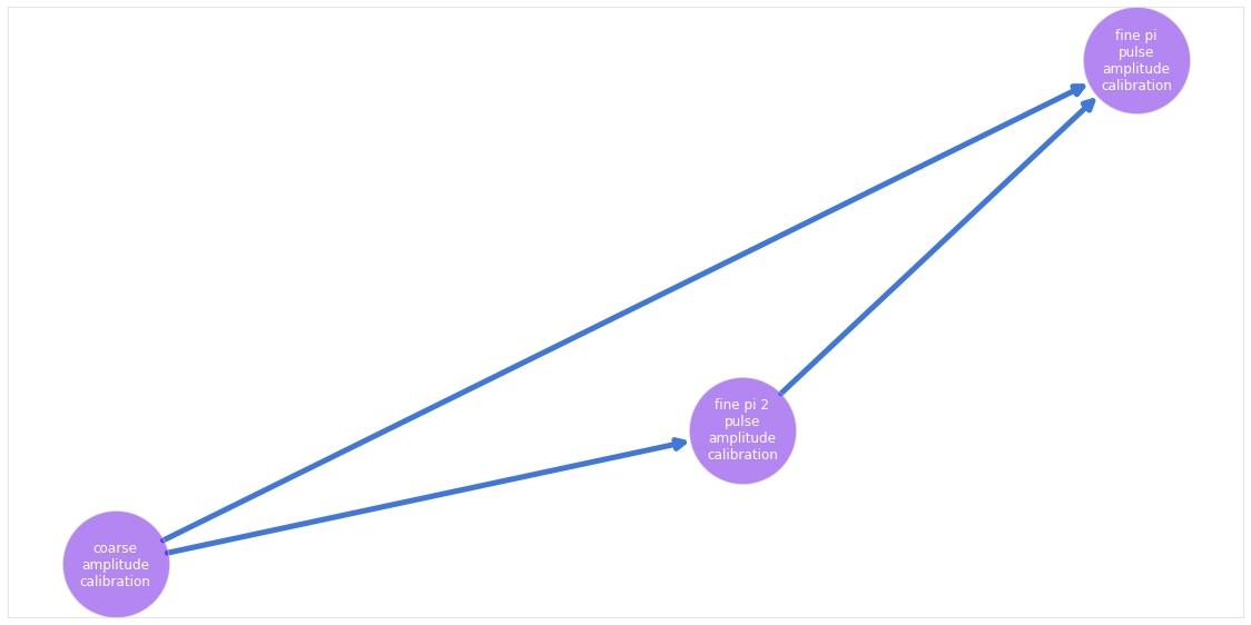
# Ask the scheduler to execute the node on which all the other nodes
# depend. As the other calibrations haven't been performed yet, this will
# trigger their execution as well.
final_node = calibration_graph.get_node("fine_pi_pulse_amplitude_calibration")

calibration_graph.execute(final_node)
# Print final value of the amplitude variables.
for variable in ["pi_pulse_amplitude", "pi_2_pulse_amplitude"]:
print(f"{variable:20s}: {calibration_graph.get_variable(variable).get()}")pi_pulse_amplitude : [0.78248268]
pi_2_pulse_amplitude: [0.39159034]
original_pi_2_amplitude = calibration_graph.get_variable("pi_2_pulse_amplitude").get()# Check the results by plotting the inifidelity after
# several repetitions of the experiment.
repetitions = np.array([4, 16, 24, 36, 48])
pi_pulse_data = []
pi_2_pulse_data = []
for repetition in repetitions:
pi_2_pulse_data.append(
backend.pi_2_pulse_experiment(
amplitude=original_pi_2_amplitude,
drag=np.array([0]),
repetition_count=repetition,
shot_count=100000,
)
)
pi_pulse_data.append(
backend.pi_pulse_experiment(
amplitude=calibration_graph.get_variable("pi_pulse_amplitude").get(),
drag=np.array([0]),
repetition_count=repetition,
shot_count=100000,
)
)
plt.xlabel("Gate repetitions")
plt.ylabel("Infidelity")
plt.plot(repetitions, pi_2_pulse_data, label=r"$\pi$/2 pulse")
plt.plot(repetitions, pi_pulse_data, label=r"$\pi$ pulse")
plt.legend()
plt.show()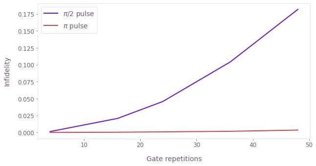
Example: Add custom closed-loop step to finely tune the $\pi/2$ pulse
The scheduler also allows you to customize your calibrations, either by adding to the existing predefined graphs, or starting new graphs from scratch.
In the example below, we show how to add a simple closed-loop optimization at the end of the predefined graph used in the other calibration. The closed-loop optimization will attempt to go further than the previously established calibration procedures by also calibrating the DRAG parameter of the Gaussian $\pi/2$ pulse.
We show also how to visualize the graph after this addition, and to re-run the calibration, this time with the additional node also present.
pi_2_pulse_amplitude = calibration_graph.get_variable("pi_2_pulse_amplitude")
drag_bound = 320e-9
pi_2_pulse_drag = calibration_graph.create_variable(
    name="pi_2_pulse_drag",
    initial_value=np.array([0]),
    lower_bound=-drag_bound,
    upper_bound=drag_bound,
)
# Define custom calibration function.
def sample_closed_loop_calibration(_calibration_graph):
sample_point_count = 51
# Gets the current value of the pi/2 pulse amplitude, use it to
# generate a series of test points.
initial_parameters = np.array(
[
np.clip(np.linspace(0.85, 1.15, sample_point_count), 0, 1)
* pi_2_pulse_amplitude.get(),
np.linspace(-drag_bound, drag_bound, sample_point_count),
]
).T
# Define a simulated experiment applying the pi/2 pulse
# different numbers of repetitions.
def _experiment(input_array):
amplitudes = input_array[:, 0]
drag_parameters = input_array[:, 1]
experiment_data = {
count: backend.pi_2_pulse_experiment(
amplitude=amplitudes,
drag=drag_parameters,
shot_count=10000,
repetition_count=count,
)
for count in [5, 6, 7, 8]
}
return np.squeeze(
2 * np.abs(0.5 - experiment_data[5])
+ np.abs(1 - experiment_data[6])
+ 2 * np.abs(0.5 - experiment_data[7])
+ np.abs(experiment_data[8])
)
# Run a simple closed-loop optimization of the pi/2 pulse.
amplitude_bounds = np.clip(
np.array([0.85, 1.15]) * pi_2_pulse_amplitude.get(), 0, 1
)
bounds = np.array([amplitude_bounds, [-drag_bound, drag_bound]])
result = bo.closed_loop.optimize(
cost_function=_experiment,
initial_parameters=initial_parameters,
optimizer=bo.closed_loop.GaussianProcess(
bounds=bo.closed_loop.Bounds(bounds), seed=7
),
max_iteration_count=10,
)
# Gather the best parameter of the calibration.
best_parameters = result["parameters"]
pi_2_pulse_amplitude.set(np.array([best_parameters[0]]))
pi_2_pulse_drag.set(np.array([best_parameters[1]]))
return es.CalibrationStatus.PASS
# Add a new node to the end of the previously-defined graph.
new_node = calibration_graph.create_node(
name="closed_loop_calibration",
dependencies=[final_node],
calibration_function=sample_closed_loop_calibration,
)
# Visualize the updated graph.
calibration_graph.visualize()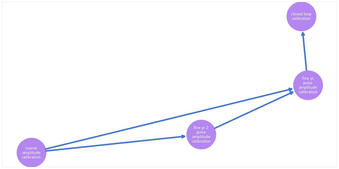
# Run graph this time with the new node.
# As the previous calibrations have already been performed,
# the scheduler only runs the new node.
calibration_graph.execute(new_node)
Running closed loop optimization
-----------------------------------------------
Optimizer : Gaussian process
Number of test points : 51
Number of parameters : 2
-----------------------------------------------
Calling cost function…
Initial best cost: 2.387e-01
Running optimizer…
Calling cost function…
Best cost after 1 iterations: 2.387e-01
Running optimizer…
Calling cost function…
Best cost after 2 iterations: 2.387e-01
Running optimizer…
Calling cost function…
Best cost after 3 iterations: 2.387e-01
Running optimizer…
Calling cost function…
Best cost after 4 iterations: 2.387e-01
Running optimizer…
Calling cost function…
Best cost after 5 iterations: 2.387e-01
Running optimizer…
Calling cost function…
Best cost after 6 iterations: 2.387e-01
Running optimizer…
Calling cost function…
Best cost after 7 iterations: 2.387e-01
Running optimizer…
Calling cost function…
Best cost after 8 iterations: 2.387e-01
Running optimizer…
Calling cost function…
Best cost after 9 iterations: 6.780e-02
Running optimizer…
Calling cost function…
Best cost after 10 iterations: 6.780e-02
Maximum iteration count reached. Stopping the optimization.
# Print updated values of the pulse variables.
for variable in ["pi_pulse_amplitude", "pi_2_pulse_amplitude", "pi_2_pulse_drag"]:
    print(f"{variable:20s}: {calibration_graph.get_variable(variable).get()}")
pi_pulse_amplitude : [0.78248268]
pi_2_pulse_amplitude: [0.40090931]
pi_2_pulse_drag : [-1.95523041e-08]
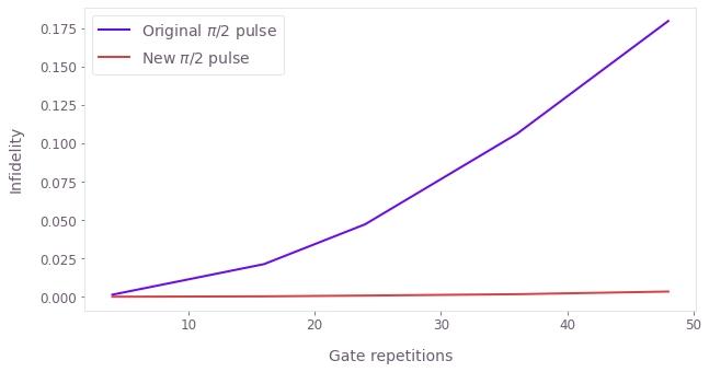
# Check the results by plotting the inifidelity after
# several repetitions of the experiment.

repetitions = np.array([4, 16, 24, 36, 48])

original_pi_2_pulse_data = []
new_pi_2_pulse_data = []

for repetition in repetitions:
    original_pi_2_pulse_data.append(
        backend.pi_2_pulse_experiment(
            amplitude=original_pi_2_amplitude,
            drag=np.array([0]),
            repetition_count=repetition,
            shot_count=100000,
        )
    )
    new_pi_2_pulse_data.append(
        backend.pi_2_pulse_experiment(
            amplitude=calibration_graph.get_variable("pi_2_pulse_amplitude").get(),
            drag=calibration_graph.get_variable("pi_2_pulse_drag").get(),
            repetition_count=repetition,
            shot_count=100000,
        )
    )

plt.xlabel("Gate repetitions")
plt.ylabel("Infidelity")

plt.plot(repetitions, original_pi_2_pulse_data, label=r"Original $\pi$/2 pulse")
plt.plot(repetitions, new_pi_2_pulse_data, label=r"New $\pi$/2 pulse")

plt.legend()
plt.show()