How to automate calibration of control hardware
Calibrate RF control channels for maximum pulse performance
Boulder Opal outputs various control solutions that can be used to define operations in real control hardware. Here we will show you how to automate the process of calibrating the RF or microwave channels used to implement controls for real quantum hardware in order to achieve maximum-fidelity operations. The calibration process allows translation of the pulse that you define at the Hamiltonian level to a useful control applied to a device, and also provides a means to account for small hardware imperfections.
In this notebook we outline the general approach, demonstrate the calibration procedure using IBM hardware, and experimentally validate the procedure's performance using complex optimized gates formatted for Qiskit. For concreteness we focus on examples calibrating single-channel RF drives. However these approaches can be generalized for the calibration of any control signal used in any quantum hardware or control electronics.
This user guide sets up a closed-loop optimization loop by directly calling the Boulder Opal API. The closed-loop module can help you simplify the optimization workflow. For more information, see this tutorial or this user guide.
IQ channel calibration formulation and objective
Most control solutions involve programming a complex time-varying control that can be written using a traditional $IQ$ decomposition familiar in RF engineering:
\begin{align} \gamma(t) &= \Omega(t) e^{i\phi(t)} = I(t) + i Q(t) \end{align}
using the $IQ$ decomposition
\begin{align} I = \Omega \cos(\phi),\\ Q = \Omega \sin(\phi),\\ |\gamma|\le\Omega_\text{max}. \end{align}
The central calibration task is to determine the relationship between these dimensionful units and the dimensionless variables employed in programming a hardware device, $A = A_I + i A_Q$. For instance on the IBM hardware these variables take values $A_{I,Q} \in [-1,1]$, although these may alternatively be, for example, integers representing a 16-bit number. This calibration must be performed with sufficient fidelity to allow the implementation of high-fidelity controls which faithfully represent the intended Hamiltonian terms. We break this into two steps below.
Summary workflow
1. Coarse IQ channel calibration
Coarsely calibrate the drive amplitude by measuring any recognizable system response (such as Rabi oscillations) using square pulses with variable amplitude or length. Repeat for different square-pulse settings to produce a coarse map of $(A_I, A_Q) \longleftrightarrow (I, Q)$.
This procedure can identify nonlinear regimes that may required pre-distortion and also mitigates the $\mathrm{mod} (2\pi)$ calibration ambiguity that inhibits direct automation in systems exhibiting periodicity (for example, Rabi oscillations). Performing an initial coarse calibration of system response to a single pulse stimulus permits appropriate bounding of parameter spaces for automation.
The workflow for this coarse calibration is as follows:
- Run Rabi experiments for a range of pulse amplitudes $A_I$.
- Fit the resulting oscillations to obtain the Rabi rates $I$ for each $A_I$.
- Interpolate the results to establish the mapping $A_I \longleftrightarrow I$.
A detailed implementation of this procedure on the IBM Quantum hardware is presented in the example below.
2. Fine IQ channel calibration
Use automated closed-loop optimization (or scripting) to determine two additional scaling factors $(S_{amp}, S_{rel})$
\begin{align} \gamma(t) = S_{amp} (S_{rel} A_I(t) + i A_Q(t)). \end{align}
The $S_{rel}$ factor allows you to account for relative differences between the designed and the actual values of $I$ and $Q$ reaching the device, while $S_{amp}$ accounts for an absolute amplitude scaling. Starting values of these fine-tuning scaling factors should be $\approx1$ as $S_{amp} = S_{rel} = 1$ corresponds to the values obtained from the previous coarse calibration.
In the calibration procedure, error amplification may be employed in order to accurately discern small differences in the impact of $S_{amp}$ and $S_{rel}$. This is easily achieved by employing gate repetition—for simplicity you should choose multiples of the target gate repetition to return a net operation the same as a single operation.
Determining $(S_{amp}, S_{rel})$ is in general sufficient to produce high-fidelity implementation of an arbitrary control operation. We note that further calibration may require system identification to determine unknown signal distortion via transmission lines.
Example: Calibration of single-qubit gates on IBM hardware
In the following we will perform these steps using IBM hardware and demonstrate a series of verification experiments to illustrate the benefits of this approach.
Our target will be the efficient calibration of the control lines used to implement a single-qubit gate. In the first section of this example, you'll learn how to perform coarse calibration of Rabi rates on a hardware device—in this case from IBM. With this initial information we will then show how to use automated closed-loop optimization in order to perform fine calibration. As an alternative we will also present a simpler but less efficient approach based on scripting to perform the same fine calibration. We will conclude with pulse-repetition experiments that illustrate the efficacy of the calibration approach outlined above.
Some cells in this notebook require an IBM Quantum account to execute correctly. If you want to run them, please go to IBM Quantum Platform to set up an account.
Coarse calibration of Rabi rates
We begin by identifying the relationship $(A_I, A_Q) \longleftrightarrow (I, Q)$ by performing experiments on IBM hardware, accessed using Qiskit pulse (analog-layer programming). In all circumstances Qiskit-specific code can be replaced with your own hardware-programming scripts.
# Imports and initialization
import boulderopal as bo
import jsonpickle
import matplotlib.pyplot as plt
import numpy as np
import qctrlvisualizer as qv
from scipy import interpolate
from scipy.optimize import curve_fit

# Mute messages from Boulder Opal calls.
bo.cloud.set_verbosity("QUIET")

# Choose to run experiments or to use saved data
use_saved_data = True

# Plotting parameters
plt.style.use(qv.get_qctrl_style())
markers = {"x": "x", "y": "s", "z": "o"}
lines = {"x": "--", "y": "-.", "z": "-"}

# Definition of operators and functions to be calibrated
sigma_z = np.array([[1.0, 0.0], [0.0, -1.0]], dtype=complex)
sigma_x = np.array([[0.0, 1.0], [1.0, 0.0]], dtype=complex)
sigma_y = np.array([[0.0, -1.0j], [1.0j, 0.0]], dtype=complex)
X90_gate = np.array([[1.0, -1j], [-1j, 1.0]], dtype=complex) / np.sqrt(2)
bloch_basis = ["x", "y", "z"]


# Initialize Qiskit parameters and IBM hardware
import warnings

warnings.simplefilter("ignore")
use_IBM = False

if use_IBM is True:
    # IBM Quantum imports
    import qiskit as qs

    # IBM credentials and backend selection
    qs.IBMQ.enable_account("your IBM token")
    provider = qs.IBMQ.get_provider(
        hub="your hub", group="your group", project="your project"
    )
    backend = provider.get_backend("ibmq_jakarta")
    backend_defaults = backend.defaults()
    backend_config = backend.configuration()

    # Backend properties
    dt = backend_config.dt
    print(f"Hardware sampling time: {dt/1e-9} ns")

    qubit_freq_est = []
    for qubit in backend_config.meas_map[0]:
        qubit_freq_est.append(backend_defaults.qubit_freq_est[qubit])
        print(f"Qubit [{qubit}] frequency estimate: {qubit_freq_est[qubit]/1e9} GHz")
# Define functions used in performance verification.
def save_variable(file_name, var):
"""
Save a single variable to a file using jsonpickle.
"""
with open(file_name, "w+") as file:
file.write(jsonpickle.encode(var))
def load_variable(file_name):
"""
Load a variable from a file encoded with jsonpickle.
"""
with open(file_name, "r+") as file:
return jsonpickle.decode(file.read())
def fit_function_bounds(x_values, y_values, function, bound_values):
"""
Fit some data to a given function.
"""
fitparams, conv = curve_fit(function, x_values, y_values, bounds=bound_values)
y_fit = function(x_values, *fitparams)
return fitparams, y_fit
def moving_average(x, w):
"""
Calculate moving average of a sequence.
"""
return np.convolve(x, np.ones(w), "valid") / w# Setting up calibration experiments
qubit = 0
dt = 2 / 9 * 1e-9
num_shots_per_point = 1024
# Variable square pulse amplitudes
pulse_amp_array = np.linspace(0.05, 0.2, 7)
# Variable square pulse durations
pulse_times = [
16 * (4 + np.arange(0, int(3.6 / (amplitude)), 1)) for amplitude in pulse_amp_array
]
# Experimental setup
if use_saved_data is False:
backend.properties(refresh=True)
qubit_frequency_updated = backend.properties().qubit_property(qubit, "frequency")[0]
meas_map_idx = None
for i, measure_group in enumerate(backend_config.meas_map):
if qubit in measure_group:
meas_map_idx = i
break
assert meas_map_idx is not None, f"Couldn't find qubit {qubit} in the meas_map!"
inst_sched_map = backend_defaults.instruction_schedule_map
measure_schedule = inst_sched_map.get("measure", qubits=[qubit])
drive_chan = qs.pulse.DriveChannel(qubit)
rabi_programs_dic_I = {}
for idx, pulse_amplitude in enumerate(pulse_amp_array):
rabi_schedules_I = []
for duration_pulse in pulse_times[idx]:
drive_pulse = qs.pulse.library.gaussian_square(
duration=duration_pulse,
sigma=1,
amp=pulse_amplitude,
risefall=1,
name=f"square_pulse_{duration_pulse}",
)
schedule = qs.pulse.Schedule(name=str(duration_pulse))
schedule |= (
qs.pulse.Play(drive_pulse, qs.pulse.DriveChannel(qubit))
<< schedule.duration
)
schedule += measure_schedule << schedule.duration
rabi_schedules_I.append(schedule)
rabi_experiment_program_I = qs.compiler.assemble(
rabi_schedules_I,
backend=backend,
meas_level=2,
meas_return="single",
shots=num_shots_per_point,
schedule_los=[{drive_chan: qubit_frequency_updated}]
* len(pulse_times[idx]),
)
rabi_programs_dic_I[pulse_amplitude] = rabi_experiment_program_I
# Running calibration experiments
rabi_calibration_exp_I = []
rabi_oscillations_results = []
for idx, pulse_amplitude in enumerate(pulse_amp_array):
job = backend.run(rabi_programs_dic_I[pulse_amplitude])
qs.tools.monitor.job_monitor(job)
rabi_results = job.result(timeout=120)
rabi_values = []
time_array = pulse_times[idx] * dt
for time_idx in pulse_times[idx]:
counts = rabi_results.get_counts(str(time_idx))
excited_pop = 0
for bits, count in counts.items():
excited_pop += count if bits[::-1][qubit] == "1" else 0
rabi_values.append(excited_pop / num_shots_per_point)
rabi_oscillations_results.append(rabi_values)
fit_parameters, y_fit = fit_function_bounds(
time_array,
rabi_values,
lambda x, A, rabi_freq, phi: A
* np.cos(2 * np.pi * rabi_freq * x + phi) ** 2,
(
[0.8, np.abs(pulse_amplitude * 8 * 1e7), -4],
[1, np.abs(pulse_amplitude * 11 * 1e7), 4],
),
)
rabi_calibration_exp_I.append(fit_parameters[1])
save_variable("resources/rabi_calibration_jakarta_qubit_0", rabi_calibration_exp_I)
save_variable("resources/fit_parameters", fit_parameters)
save_variable("resources/rabi_values", rabi_values)
else:
rabi_calibration_exp_I = load_variable("resources/rabi_calibration_jakarta_qubit_0")
fit_parameters = load_variable("resources/fit_parameters")
rabi_values = load_variable("resources/rabi_values")
time_array = pulse_times[-1] * dt
print("Drive amplitude:", pulse_amp_array[-1])
print("Fitted Rabi frequency [Hz]:", fit_parameters[1])
fig = plt.figure(figsize=(10, 5))
fig.suptitle("Exemplary Rabi oscillation data with fitting")
plt.xlabel("Time (s)")
plt.ylabel("Measured signal (a.u.)")
plt.scatter(time_array, np.real(rabi_values), color="black")
plt.xlim(0, time_array[-1])
plt.ylim(0, 1)
plot_times = np.linspace(0, time_array[-1], 100)
plt.plot(
plot_times,
fit_parameters[0]
* np.cos(2 * np.pi * fit_parameters[1] * plot_times + fit_parameters[2]) ** 2,
)
plt.show()Drive amplitude: 0.2
Fitted Rabi frequency [Hz]: 16000000.0000049
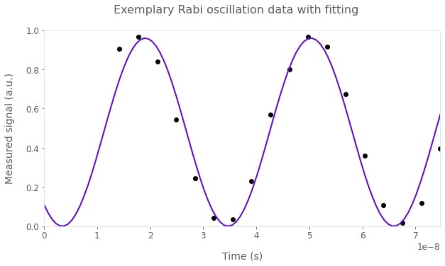
This figure shows the result of a Rabi experiment for an amplitude $A_I = 0.2$ (circles) and the correponding cosine square fit (line).
You can now collect all the $I$ values from the previous experiment and establish the correspondence between $I$ and $A_I$. This is performed in the cell below.
amplitude_interpolated_list = np.linspace(-0.2, 0.2, 100)
pulse_amp_array = np.concatenate((-pulse_amp_array[::-1], pulse_amp_array))
rabi_calibration_exp_I = np.concatenate(
    (-np.asarray(rabi_calibration_exp_I[::-1]), np.asarray(rabi_calibration_exp_I))
)
f_amp_to_rabi = interpolate.interp1d(pulse_amp_array, rabi_calibration_exp_I)
rabi_interpolated_exp_I = f_amp_to_rabi(amplitude_interpolated_list)

f_rabi_to_amp = interpolate.interp1d(
    rabi_interpolated_exp_I, amplitude_interpolated_list
)

fig = plt.figure(figsize=(10, 5))
fig.suptitle("IBMQ Jakarta: Rabi rates calibration")
plt.xlabel("Hardware input amplitude")
plt.ylabel("Rabi rate (MHz)")
plt.scatter(pulse_amp_array, rabi_calibration_exp_I * 1e-6)
plt.plot(amplitude_interpolated_list, rabi_interpolated_exp_I * 1e-6)
plt.axvline(0, color="black", linestyle="dashed")
plt.axhline(0, color="black", linestyle="dashed")
plt.show()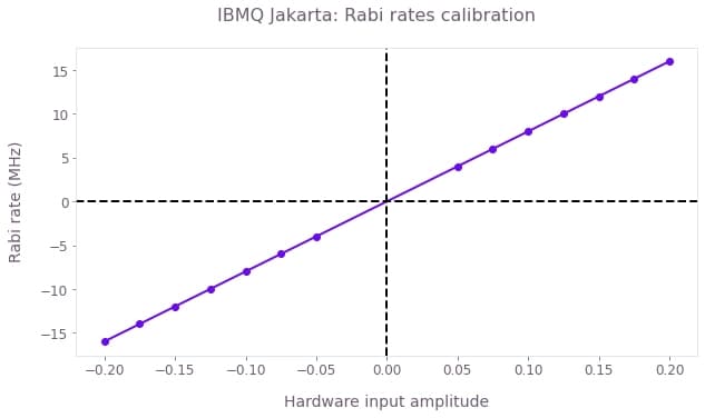
The figure shows the mapping between the Rabi rates and the dimensionless hardware input. The calibration was performed in the interval $[-0.2, 0.2]$, and the observed relationship is approximately linear. With this information we have completed the coarse calibration of Rabi rates for this specific complex drive channel.
Fine IQ calibration using an autonomous agent
We use automated closed-loop optimization to find the calibration parameters $S_{amp}, S_{rel}$ in the pulse parametrization $\gamma(t) = S_{amp} (S_{rel} A_I(t) + i A_Q(t))$ automatically. In each iteration of the procedure, the optimizer will pick a set of calibration parameters, transform the pulse, send it to the device, and receive in response measurements of the system (here measured infidelity under gate repetition) to inform the next actions of the autonomous agent. As more iterations are performed, the optimizable parameters will converge to the values that minimize the infidelity.
In what follows, the optimization bounds are set to be $S_{amp} \in [0.8,1.2]$ and $S_{rel} \in [0.8,1.2]$, that is, within $20 \%$ of the values of the initial coarse calibration step.
In each iteration of the calibration loop, you'll need to extract a measurement to be returned to the optimizer. The cost function may be created in a manner that best suits your hardware; we recommend measuring gate infidelity under different numbers of repetition $N$ and then averaging the fidelities for each value of gate repetition. Using repetitions amplifies the error in each gate, and averaging over different repetition numbers mitigates pathologies arising for specific experimental conditions. For the $X_{\pi/2}$ pulses, you can use $N = (1 + 4n)$ repetitions with $n \in \{0, 1 \cdots \}$ so that the Bloch vector always ends up in the same point if the pulse is perfect.
The functions in the cell below show how to do this using Qiskit. If you want to deploy this calibration in your own experiment, you'll need to modify these functions accordingly.
error_mitigation = True


def run_ibm_experiments(control, calibration_pairs, repetitions, qubit):
    I_values = control["I"]["values"]
    Q_values = control["Q"]["values"]

    schedules = []
    for scal in calibration_pairs:
        scaled_waveform = (I_values * scal[0] + 1j * Q_values) * scal[1]
        control_pulse = qs.pulse.Play(
            qs.pulse.library.Waveform(scaled_waveform), qs.pulse.DriveChannel(qubit)
        )
        for meas_basis in bloch_basis:
            for repetition in repetitions:
                schedule = qs.pulse.Schedule(
                    name=f"pulse_scal_{scal}_reps_{repetition}_basis_{meas_basis}"
                )
                for reps in np.arange(repetition):
                    schedule += control_pulse
                if meas_basis == "x":
                    schedule += inst_sched_map.get("u2", [qubit], P0=0.0, P1=np.pi)
                    schedule += measure_schedule << schedule.duration
                if meas_basis == "y":
                    schedule += inst_sched_map.get("u2", [qubit], P0=0.0, P1=np.pi / 2)
                    schedule += measure_schedule << schedule.duration
                if meas_basis == "z":
                    schedule |= measure_schedule << schedule.duration
                schedules.append(schedule)

    # Running the jobs
    job = qs.execute(schedules, backend, shots=num_shots_per_point)
    print("Job id:", job.job_id())
    qs.tools.monitor.job_monitor(job)
    exp_results = job.result(timeout=120)

    return exp_results


def extract_results(results, calibration_pairs):
    idx = 0
    pairs_results = []
    if error_mitigation:
        results = measurementFilter.apply(results)

    for scaling_pair in calibration_pairs:
        basis_results = []
        for meas_basis in bloch_basis:
            rep_results = []
            for number_of_repetitions in repetitions:
                count = qs.ignis.verification.marginal_counts(
                    results.get_counts()[idx], meas_qubits=[0]
                )
                excited_pop = 0
                idx += 1
                excited_pop += count["1"]
                rep_results.append(excited_pop / num_shots_per_point)
            basis_results.append(rep_results)
        pairs_results.append(1 - 2 * np.asarray(basis_results))
    calibration_data = np.asarray(pairs_results)

    # Infidelities for repetition experiments
    target_bloch = np.array([0, -1, 0])
    bloch_vectors = np.array(
        [
            np.array([calibration_data[idx, :, rep] for rep in range(len(repetitions))])
            for idx in range(len(calibration_pairs))
        ]
    )
    bloch_infidelity = 1 - ((1 + np.dot(bloch_vectors, target_bloch)) / 2) ** 2

    cost_infidelity = np.average(bloch_infidelity, axis=1)
    print("Best cost in this step:", np.min(cost_infidelity))

    return cost_infidelity


def conductErrorMitigation(shots):
    """Measure the state preparation and measurement error"""

    cal_circuits, state_labels = qs.ignis.mitigation.measurement.complete_meas_cal(
        qubit_list=np.arange(7), circlabel="MeasErrMitCal"
    )

    cal_job = qs.execute(cal_circuits, backend=backend, shots=shots)
    qs.tools.monitor.job_monitor(cal_job)
    cal_results = cal_job.result()

    meas_fitter = qs.ignis.mitigation.measurement.CompleteMeasFitter(
        cal_results, state_labels
    )

    # Set the object's measurementFilter here
    meas_filter = meas_fitter.filter

    ErrorMitigationComplete = True
    return meas_filter


if use_saved_data is False and error_mitigation:
    SPAMshots = 1024 * 4
    measurementFilter = conductErrorMitigation(shots=SPAMshots)
Here, you'll calibrate a specific control pulse using the coarse calibration information performed above. The cell below imports a specific pulse to calibrate and plots the waveform. In the Designing noise-robust single-qubit gates for IBM Qiskit application note you'll find a detailed explanation on how to construct robust pulses for superconducting qubit systems.
# Import pulses
gate_schemes = load_variable("resources/pulse_amplitude_robust")

# Extract pulse properties
number_of_segments = {}
duration_int = {}
duration = {}
segment_scale = {}
waveform = {}
for scheme_name, control in gate_schemes.items():
    number_of_segments[scheme_name] = len(control["I"]["durations"])
    duration[scheme_name] = sum(control["I"]["durations"])
    duration_int[scheme_name] = int(round(duration[scheme_name] / dt))
    segment_scale[scheme_name] = (
        duration_int[scheme_name] / number_of_segments[scheme_name]
    )
    I_values = control["I"]["values"] / 2 / np.pi
    Q_values = control["Q"]["values"] / 2 / np.pi
    A_I_values = np.repeat(f_rabi_to_amp(I_values), segment_scale[scheme_name])
    A_Q_values = np.repeat(f_rabi_to_amp(Q_values), segment_scale[scheme_name])
    waveform[scheme_name] = A_I_values + 1j * A_Q_values

# Plot pulses
for scheme_name, gate in gate_schemes.items():
    qv.plot_controls(gate)
    plt.suptitle(scheme_name)
    plt.show()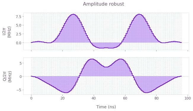
The above plots display I and Q components of the microwave drive on the qubit for an amplitude robust pulse that performs a $\pi/2$ rotation around the $x$ axis (an $X_{\pi/2}$ gate). Note that the values of the pulse waveform are given in natural units of MHz.
# Invoke the pulse described above in the calibration procedure
pulse_duration = dt * waveform["Amplitude robust"].shape[0]
pulse_to_calibrate = {
    "I": {
        "durations": np.repeat(pulse_duration, waveform["Amplitude robust"].shape[0]),
        "values": np.real(waveform["Amplitude robust"]),
    },
    "Q": {
        "durations": np.repeat(pulse_duration, waveform["Amplitude robust"].shape[0]),
        "values": np.imag(waveform["Amplitude robust"]),
    },
}
The next cell sets up the automated optimization and runs the calibration loop. Here you will directly set the optimization cost as the average infidelity for multiple repetitions, streamlining the calibration process by requiring less human intervention.
To minimize the number of API calls to the IBM Quantum device, the calibration procedure will make use of the batching feature of Boulder Opal (see How to automate closed-loop hardware optimization for more information). By setting test_point_count to 5, you'll send five independent jobs under a single request in the queue. In this way, the optimizer will use the result from five different sets of calibration parameters in each iteration.
if use_saved_data:
    best_cost_array = load_variable("resources/best_cost_array_jakarta_June_8")
    best_param_array = load_variable("resources/best_control_array_jakarta_June_8")
    print(f"Infidelity: {best_cost_array[-1]}")
    print(f"Calibration parameters: {best_param_array[-1]}")
else:
    repetitions = np.arange(5, 42, 12)
    relative_bounds = (0.8, 1.2)
    amplitude_bounds = (0.8, 1.2)
    test_point_count = 5

    calibration_result = {}
    best_cost_array = []
    best_param_array = []

    # Create random pairs for initial batch
    rng = np.random.default_rng()
    parameter_set = [
        [
            rng.uniform(relative_bounds[0], relative_bounds[1]),
            rng.uniform(amplitude_bounds[0], amplitude_bounds[1]),
        ]
        for idx in np.arange(test_point_count)
    ]

    # Run the experiment with the initial random calibration parameters
    exp_results = run_ibm_experiments(
        pulse_to_calibrate, parameter_set, repetitions, qubit
    )
    cost_results = extract_results(exp_results, parameter_set)

    # OPTIMIZATION SETUP
    bounds = bo.closed_loop.Bounds(np.array([relative_bounds, amplitude_bounds]))
    optimizer = bo.closed_loop.GaussianProcess(bounds=bounds, seed=0)

    best_cost, best_controls = min(
        zip(cost_results, parameter_set), key=lambda params: params[0]
    )
    optimization_count = 0

    best_cost_array.append(best_cost)
    best_param_array.append(best_controls)

    # Run the optimization loop until the cost is sufficiently small or when it reaches 10 steps
    idx = 0
    while best_cost > 0.005 and idx <= 10:
        # Print the current best cost.
        optimization_steps = (
            "optimization step" if optimization_count == 1 else "optimization steps"
        )
        print(
            f"Best infidelity after {optimization_count} Boulder Opal {optimization_steps}: {best_cost}"
        )

        # Organize the experiment results into the proper input format
        results = bo.closed_loop.Results(
            parameters=np.asarray(parameter_set),
            cost=cost_results,
            cost_uncertainty=np.repeat(0.1, len(cost_results)),
        )

        # Call the automated closed-loop optimizer and obtain the next set of test points
        optimization_result = bo.closed_loop.step(
            optimizer=optimizer, results=results, test_point_count=test_point_count
        )
        optimization_count += 1

        # Organize the data returned by the automated closed-loop optimizer
        parameter_set = optimization_result["test_points"]
        optimizer = optimization_result["state"]

        # Obtain experiment results that the automated closed-loop optimizer requested
        exp_results = run_ibm_experiments(
            pulse_to_calibrate, parameter_set, repetitions, qubit
        )
        cost_results = extract_results(exp_results, parameter_set)

        params_array.append(parameter_set)

        # Record the best results after this round of experiments
        cost, controls = min(
            zip(cost_results, parameter_set), key=lambda params: params[0]
        )

        if cost < best_cost:
            best_cost = cost
            best_controls = controls
        idx += 1
        best_cost_array.append(best_cost)
        best_param_array.append(best_controls)
        print("Best parameters:", best_controls)

    # Print final best cost.
    print(f"Infidelity: {best_cost}")
    print(f"Calibration parameters: {best_controls}")
    calibration_result[qubit] = best_controls
Infidelity: 0.00827659524514815
Calibration parameters: [1.02161937 1.04297263]
# Plotting
qv.plot_cost_histories(best_cost_array, initial_iteration=0)
plt.suptitle("Convergence of automated pulse calibration")
plt.show()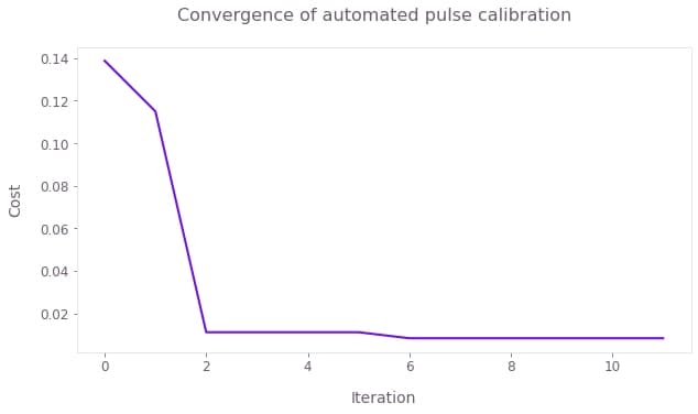
Gate infidelity averaged for multiple repetitions of the pulses (5, 17, 29, and 41, in this case) as a function of the number of optimization steps. The calibration converges after a couple of steps, with the cost below $1\%$, after readout error mitigation. The final calibration parameters are $(S_{amp}, S_{rel}) = (1.043, 1.022)$.
Fine IQ calibration using scripted parametric scans over $S_{rel}$ and $S_{amp}$
An alternative approach to performing fine calibration involves the execution of scripted scans over the parameters $(S_{amp}, S_{rel})$. This approach may be used as a manual diagnostic or in cases where automated optimization is not accessible. The procedure is described below.
-
Using two sequences with different numbers of pulse repetitions ($N_1$ and $N_2$), perform experiments where you measure gate infidelity as a function of $S_{rel}\approx 1$, scanning over a narrow range.
-
Find the value of the scaling factor, $S_{rel}$, that minimizes the infidelity for both repetition numbers. You could be tempted to use a single repetition number $N$ to speed up your calibration but this is not advisable. Note that, if you pick $N$ that is too small, there will be little variation of the infidelity with $S_{rel}$ and your calibration would be inaccurate. If you select $N$ that is too large, you may see multiple infidelity minima as small changes in $S_{rel}$ can lead to full rotations in the Bloch sphere. In this case, you may be selecting the wrong scaling factor. Using two values allows you to find a single scaling that best calibrates your pulse.
-
Repeat step 2, now fixing the value of $S_{rel}$ found to minimize infidelity in the previous step and scaning $S_{amp}$. Again, find the scaling factor that minimizes the infidelity for both pulse repetition numbers.
The following cell executes steps 1 and 2 above for the IBM device using an automated routine to identify the appropriate value of $S_{rel}$. Here we select $N_1 = 49$ and $N_2 =101$.
repetitions = np.array([49, 101])
scalings = np.linspace(0.95, 1.05, 50)

if use_saved_data is False:
    pulse_program = {}
    for scheme_name in gate_schemes.keys():
        schedules = []
        for meas_basis in bloch_basis:
            for repetition in repetitions:
                for scaling_factor_I in scalings:
                    Ival = np.real(waveform[scheme_name]) * scaling_factor_I
                    Qval = np.imag(waveform[scheme_name])
                    scaled_waveform = Ival + 1j * Qval
                    control_pulse = qs.pulse.Play(
                        qs.pulse.library.Waveform(scaled_waveform), drive_chan
                    )
                    schedule = qs.pulse.Schedule(
                        name=f"pi_pulse_scal_{scaling_factor_I}_reps_{repetition}_basis_{meas_basis}"
                    )
                    for reps in np.arange(repetition):
                        schedule += control_pulse
                    if meas_basis == "x":
                        schedule += inst_sched_map.get("u2", [0], P0=0.0, P1=np.pi)
                        schedule += measure_schedule << schedule.duration
                    if meas_basis == "y":
                        schedule += inst_sched_map.get("u2", [0], P0=0.0, P1=np.pi / 2)
                        schedule += measure_schedule << schedule.duration
                    if meas_basis == "z":
                        schedule |= measure_schedule << schedule.duration
                    schedules.append(schedule)
        pulse_program[scheme_name] = qs.compiler.assemble(
            schedules,
            backend=backend,
            meas_level=2,
            meas_return="single",
            shots=num_shots_per_point,
            schedule_los=[{drive_chan: qubit_frequency_updated}]
            * (repetitions.shape[0])
            * (scalings.shape[0])
            * 3,
        )

    # Running the jobs
    exp_results = {}
    for scheme_name in gate_schemes.keys():
        print("Control Scheme:", scheme_name)
        job = backend.run(pulse_program[scheme_name])
        print("Job id:", job.job_id())
        qs.tools.monitor.job_monitor(job)
        exp_results[scheme_name] = job.result(timeout=120)

    # Extract results
    I_calibration_data = {}
    for scheme_name, results in exp_results.items():
        print(scheme_name)
        idx = 0
        result_bloch = []
        for meas_basis in bloch_basis:
            full_res = []
            for idx_rep, number_of_repetitions in enumerate(repetitions):
                rep_res = []
                for scaling_factor in scalings:
                    counts = results.get_counts()[idx]
                    excited_pop = 0
                    idx += 1
                    for bits, count in counts.items():
                        excited_pop += count if bits[::-1][qubit] == "1" else 0
                    rep_res.append(excited_pop / num_shots_per_point)
                full_res.append(rep_res)
            result_bloch.append(1 - 2 * np.asarray(full_res))
        I_calibration_data[scheme_name] = np.asarray(result_bloch)

    save_variable(
        "resources/relative_calibration_data_jakarta_qubit_0", I_calibration_data
    )

else:
    I_calibration_data = load_variable(
        "resources/relative_calibration_data_jakarta_qubit_0"
    )

# Infidelities for repetition experiments
target_bloch = np.array([0, -1, 0])
bloch_infidelity = {}
for scheme_name in gate_schemes.keys():
    bloch_vectors = np.array(
        [
            np.array(
                [
                    I_calibration_data[scheme_name][:, rep, idx]
                    for idx in range(scalings.shape[0])
                ]
            )
            for rep in range(repetitions.shape[0])
        ]
    )
    bloch_infidelity[scheme_name] = (
        1 - ((1 + np.dot(bloch_vectors, target_bloch)) / 2) ** 2
    )

# Plotting
fig, axs = plt.subplots(1, len(gate_schemes.keys()), figsize=(10, 5), squeeze=False)
fig.suptitle("Relative scaling calibration from pulse repetitions", y=1)

# Find the optimal value of S_rel by averaging data for N_1 and N_2 together and finding the minimum infidelity.
best_scaling_I = {}
average_infidelity = {}
for idx, scheme_name in enumerate(gate_schemes.keys()):
    ax = axs[0][idx]
    infidelity_smoothed = []
    for idx, pulse_repetition in enumerate(repetitions):
        infidelity_smoothed.append(
            moving_average(bloch_infidelity[scheme_name][idx, :], 3)
        )
        ax.set_title(f"Control: {scheme_name}")
        ax.scatter(
            scalings,
            bloch_infidelity[scheme_name][idx, :],
            label=f"Infidelity data for {pulse_repetition} pulse repetitions",
        )
        ax.plot(
            scalings[1:-1],
            infidelity_smoothed[-1],
            label=f"Smoothed infidelity for {pulse_repetition} pulse repetitions",
        )
        ax.set_xlabel("Relative scaling")
        ax.set_ylabel("Infidelity")

    average_infidelity[scheme_name] = np.average(infidelity_smoothed, axis=0)
    best_scaling_I[scheme_name] = scalings[
        np.argmin(average_infidelity[scheme_name]) + 1
    ]
    ax.plot(
        scalings[1:-1],
        average_infidelity[scheme_name],
        label="Average infidelity",
        c="k",
    )
    ax.axvline(best_scaling_I[scheme_name], ls="--")
    ax.text(
        scalings[np.argmin(infidelity_smoothed) + 1],
        np.max(infidelity_smoothed),
        "Best $S\_{rel}$: %.3f" % scalings[np.argmin(infidelity_smoothed) + 1],
        fontsize=14,
    )
    ax.set_ylim(0, 1.05)
ax.legend(loc="upper left", bbox_to_anchor=(1, 1))
plt.show()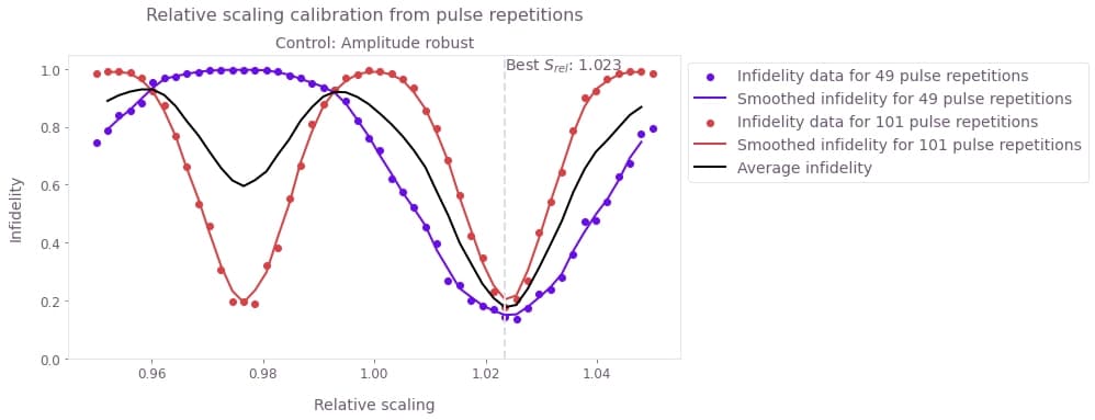
Infidelity as a function of $S_{rel}$ for 49 and 101 repetitions of the pulse. The solid lines are a moving average of the experimental results (symbols) using the values from 3 points. The black solid line is the average between the 49 and 101 repetitions experiments. The scaling factor that you should use when calibrating your pulse is the one that minimizes the average infidelity.
The following cell now performs step 3 for $S_{amp}$.
repetitions = np.array([49, 101])
scalings = np.linspace(0.95, 1.05, 50)

if use_saved_data is False:
    pulse_program = {}
    for scheme_name in gate_schemes.keys():
        schedules = []
        for meas_basis in bloch_basis:
            for repetition in repetitions:
                for scaling_factor in scalings:
                    scaled_waveform = (
                        np.real(waveform[scheme_name]) * best_scaling_I[scheme_name]
                        + 1j * np.imag(waveform[scheme_name])
                    ) * scaling_factor
                    control_pulse = qs.pulse.Play(
                        qs.pulse.library.Waveform(scaled_waveform), drive_chan
                    )
                    schedule = qs.pulse.Schedule(
                        name=f"pi_pulse_scal_{scaling_factor}_reps_{repetition}_basis_{meas_basis}"
                    )
                    for reps in np.arange(repetition):
                        schedule += control_pulse
                    if meas_basis == "x":
                        schedule += inst_sched_map.get("u2", [0], P0=0.0, P1=np.pi)
                        schedule += measure_schedule << schedule.duration
                    if meas_basis == "y":
                        schedule += inst_sched_map.get("u2", [0], P0=0.0, P1=np.pi / 2)
                        schedule += measure_schedule << schedule.duration
                    if meas_basis == "z":
                        schedule |= measure_schedule << schedule.duration
                    schedules.append(schedule)
        pulse_program[scheme_name] = qs.compiler.assemble(
            schedules,
            backend=backend,
            meas_level=2,
            meas_return="single",
            shots=num_shots_per_point,
            schedule_los=[{drive_chan: qubit_frequency_updated}]
            * (repetitions.shape[0])
            * (scalings.shape[0])
            * 3,
        )

    # Running the jobs
    exp_results = {}
    for scheme_name in gate_schemes.keys():
        print("Control Scheme:", scheme_name)
        job = backend.run(pulse_program[scheme_name])
        print("Job id:", job.job_id())
        qs.tools.monitor.job_monitor(job)
        exp_results[scheme_name] = job.result(timeout=120)

    # Extract results
    amplitude_calibration_data = {}
    for scheme_name, results in exp_results.items():
        print(scheme_name)
        idx = 0
        result_bloch = []
        for meas_basis in bloch_basis:
            full_res = []
            for idx_rep, number_of_repetitions in enumerate(repetitions):
                rep_res = []
                for scaling_factor in scalings:
                    counts = results.get_counts()[idx]
                    excited_pop = 0
                    idx += 1
                    for bits, count in counts.items():
                        excited_pop += count if bits[::-1][qubit] == "1" else 0
                    rep_res.append(excited_pop / num_shots_per_point)
                full_res.append(rep_res)
            result_bloch.append(1 - 2 * np.asarray(full_res))
        amplitude_calibration_data[scheme_name] = np.asarray(result_bloch)

    save_variable(
        "resources/amplitude_calibration_data_jakarta_qubit_0",
        amplitude_calibration_data,
    )
else:
    amplitude_calibration_data = load_variable(
        "resources/amplitude_calibration_data_jakarta_qubit_0"
    )

# Infidelities for repetition experiments
bloch_infidelity = {}
for scheme_name in gate_schemes.keys():
    bloch_vectors = np.array(
        [
            np.array(
                [
                    amplitude_calibration_data[scheme_name][:, rep, idx]
                    for idx in range(scalings.shape[0])
                ]
            )
            for rep in range(repetitions.shape[0])
        ]
    )
    bloch_infidelity[scheme_name] = (
        1 - ((1 + np.dot(bloch_vectors, target_bloch)) / 2) ** 2
    )

fig, axs = plt.subplots(1, len(gate_schemes.keys()), figsize=(10, 5), squeeze=False)
fig.suptitle("Amplitude scaling calibration from pulse repetitions", y=1)

best_scaling_amplitude = {}
average_infidelity = {}
for idx, scheme_name in enumerate(gate_schemes.keys()):
    ax = axs[0][idx]
    infidelity_smoothed = []
    for idx, pulse_repetition in enumerate(repetitions):
        infidelity_smoothed.append(
            moving_average(bloch_infidelity[scheme_name][idx, :], 5)
        )
        ax.set_title(f"Control: {scheme_name}")
        ax.scatter(
            scalings,
            bloch_infidelity[scheme_name][idx, :],
            label=f"Infidelity data for {pulse_repetition} pulse repetitions",
        )
        ax.plot(
            scalings[2:-2],
            infidelity_smoothed[-1],
            label=f"Smoothed infidelity for {pulse_repetition} pulse repetitions",
        )
        ax.set_xlabel("Amplitude scaling")
        ax.set_ylabel("Infidelity")

    average_infidelity[scheme_name] = np.average(infidelity_smoothed, axis=0)
    best_scaling_amplitude[scheme_name] = scalings[
        np.argmin(average_infidelity[scheme_name]) + 2
    ]
    ax.plot(
        scalings[2:-2],
        average_infidelity[scheme_name],
        label="Average infidelity",
        c="k",
    )
    ax.text(
        best_scaling_amplitude[scheme_name],
        0.35,
        "Best $S\_{amp}$: %.3f" % best_scaling_amplitude[scheme_name],
        fontsize=14,
    )
    ax.axvline(best_scaling_amplitude[scheme_name], ls="--")
    ax.set_ylim(0, 0.5)
ax.legend(loc="upper left", bbox_to_anchor=(1, 1))
plt.show()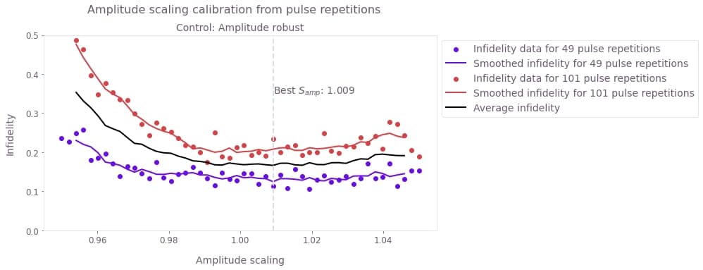
Infidelity as a function of the amplitude scaling factor $S_{amp}$. As in the previous step, the solid lines are a moving average of the experimental results (symbols), and the black solid line is the average between the two smoothed curves. In this figure, you can see that this particular pulse is mostly insensitive to the overall scaling factor as it has been designed to be robust against amplitude noise (check the Designing noise-robust single-qubit gates for IBM Qiskit application note for more information on the design of robust pulses).
Verifying calibration using a pulse-repetition experiment
Here we perform a simple experiment repeating the calibrated pulses (using the different methods above) and compare the performance. The selected pulse-repetition experiment amplifies coherent calibration errors.
repetitions = np.arange(1, 151, 4)
num_shots_per_point = 2048
calibration_results = {
    "Basic Rabi calibration": [1, 1],
    "Fine-tuned calibration": [
        best_scaling_I["Amplitude robust"],
        best_scaling_amplitude["Amplitude robust"],
    ],
    "Automated calibration": best_param_array[-1],
}

if use_saved_data is False:
    # Full pulse calibration
    calibrated_waveform = {}
    for scheme_name, scalings in calibration_results.items():
        calibrated_waveform[scheme_name] = (
            scalings[0] * np.real(waveform["Amplitude robust"])
            + 1j * np.imag(waveform["Amplitude robust"])
        ) * scalings[1]

    pulse_program = {}
    for scheme_name, calibrated_pulse in calibrated_waveform.items():
        schedules = []
        for meas_basis in bloch_basis:
            for repetition in repetitions:
                control_pulse = qs.pulse.Play(
                    qs.pulse.library.Waveform(calibrated_pulse), drive_chan
                )
                schedule = qs.pulse.Schedule(
                    name=f"pulse_reps_{repetition}_basis_{meas_basis}"
                )
                for reps in np.arange(repetition):
                    schedule += control_pulse
                if meas_basis == "x":
                    schedule += inst_sched_map.get("u2", [0], P0=0.0, P1=np.pi)
                    schedule += measure_schedule << schedule.duration
                if meas_basis == "y":
                    schedule += inst_sched_map.get("u2", [0], P0=0.0, P1=np.pi / 2)
                    schedule += measure_schedule << schedule.duration
                if meas_basis == "z":
                    schedule |= measure_schedule << schedule.duration
                schedules.append(schedule)
        pulse_program[scheme_name] = qs.compiler.assemble(
            schedules,
            backend=backend,
            meas_level=2,
            meas_return="single",
            shots=num_shots_per_point,
            schedule_los=[{drive_chan: qubit_frequency_updated}]
            * (repetitions.shape[0])
            * 3,
        )

    # Run the jobs
    exp_results = {}
    for scheme_name, program in pulse_program.items():
        print("Control Scheme:", scheme_name)
        job = backend.run(program)
        print("Job id:", job.job_id())
        qs.tools.monitor.job_monitor(job)
        exp_results[scheme_name] = job.result(timeout=120)

    # Extract results
    calibrated_pulse_performance = {}
    for scheme_name, results in exp_results.items():
        print(scheme_name)
        idx = 0
        result_bloch = []
        for meas_basis in bloch_basis:
            full_res = []
            for idx_rep, number_of_repetitions in enumerate(repetitions):
                rep_res = []
                counts = results.get_counts()[idx]
                excited_pop = 0
                for bits, count in counts.items():
                    excited_pop += count if bits[::-1][qubit] == "1" else 0
                rep_res.append(excited_pop / num_shots_per_point)
                full_res.append(rep_res)
                idx += 1
            result_bloch.append(1 - 2 * np.asarray(full_res))
        calibrated_pulse_performance[scheme_name] = np.asarray(result_bloch)

    save_variable(
        "resources/calibrated_pulse_performance_jakarta_qubit_0",
        calibrated_pulse_performance,
    )
else:
    calibrated_pulse_performance = load_variable(
        "resources/calibrated_pulse_performance_jakarta_qubit_0"
    )

# Infidelities for repetition experiments
bloch_infidelity = {}
for scheme_name, performance in calibrated_pulse_performance.items():
    bloch_vectors = performance[:, :, 0].T
    bloch_infidelity[scheme_name] = (
        1 - ((1 + np.dot(bloch_vectors, target_bloch)) / 2) ** 2
    )

# Plotting

fig = plt.figure(figsize=(10, 5))
fig.suptitle("Pulse performance after calibration")
for scheme_name, infidelity in bloch_infidelity.items():
    plt.plot(repetitions, infidelity, marker="o", label=scheme_name)
    plt.xlabel("Pulse repetition number")
    plt.ylabel("Infidelity")
    plt.ylim(0, 1.05)
plt.legend()
plt.show()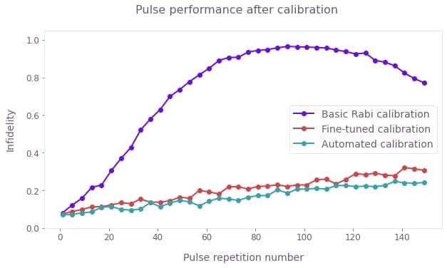
These data reveal that using only the basic coarse calibration we come close to an ideal implementation for a single pulse but the infidelity quickly worsens as the gate is repeated. The behavior observed is consistent with the onset of oscillations due to rotation errors. By contrast, both fine-calibration procedures remove this behavior and result in a decay which is approximately consistent with incoherent decay from the measured $T_{1}$ in the hardware.
