Designing noise-robust single-qubit gates for IBM Qiskit

Increasing robustness against dephasing and control noise using Boulder Opal pulses

Boulder Opal enables you to design numerically optimized controls which can improve the performance of quantum computing hardware. Specifically, robust control solutions are able to reduce sensitivity to dephasing and/or control noise, including slowly varying noise sources that arise as hardware drifts over time.

In this application note we present an entire workflow—from gate optimization through to experimental validation on IBM Quantum Hardware. We will cover:

Designing optimized dephasing-noise-robust controls using graphs
Incorporating band-limits on the optimization to produce smooth pulses
Validating performance using filter functions and quasi-static-noise-susceptibility scans
Formatting for Qiskit and experimental execution on IBM Quantum hardware.

A detailed discussion of optimized-pulse performance on IBM hardware can be found in our technical manuscript, "Error-robust quantum logic optimization using a cloud quantum computer interface", published as Phys. Rev. Applied 15, 064054 (2021). Additionally, a related workflow on Rigetti hardware can be found in the Designing noise-robust single-qubit gates for Rigetti Quil-T application note.

Some cells in this notebook require an account with IBM-Q to execute correctly. If you want to run them, please go to the IBM-Q experience to set up an account.

Imports and initialization

import time
import warnings
from pathlib import Path
import jsonpickle
import jsonpickle.ext.numpy as jsonpickle_numpy

jsonpickle_numpy.register_handlers()
import numpy as np
import scipy
import matplotlib.pyplot as plt

import qctrlvisualizer as qv

import boulderopal as bo

plt.style.use(qv.get_qctrl_style())

# Disable warning from qiskit.
warnings.filterwarnings("ignore")

# Choose to run experiments or to use saved data.
use_saved_data = True
use_IBM = False

if use_saved_data is False:
    timestr = time.strftime("%Y%m%d-%H%M%S")
    print("Time label for data saved throughout this experiment:" + timestr)
data_folder = Path("resources/")

# Parameters.
giga = 1e9
mega = 1e6
nano = 1e-9

colors = {
    "Q-CTRL": qv.QCTRL_STYLE_COLORS[0],
    "Square": qv.QCTRL_STYLE_COLORS[1],
    "IBM default X-gate": qv.QCTRL_STYLE_COLORS[2],
}

bloch_colors = {
    "x": qv.QCTRL_STYLE_COLORS[0],
    "y": qv.QCTRL_STYLE_COLORS[1],
    "z": qv.QCTRL_STYLE_COLORS[2],
}
bloch_markers = {"x": "x", "y": "s", "z": "o"}
bloch_lines = {"x": "--", "y": "-.", "z": "-"}
bloch_basis = ["x", "y", "z"]


# Auxiliary functions.
def get_detuning_scan(detunings, control):
    graph = bo.Graph()

    shift_I = graph.pwc(**control["I"])
    shift_Q = graph.pwc(**control["Q"])
    duration = np.sum(shift_I.durations)

    noise = graph.constant_pwc(
        constant=detunings, duration=duration, batch_dimension_count=1
    )

    hamiltonian = (
        shift_I * graph.pauli_matrix("X") / 2
        + shift_Q * graph.pauli_matrix("Y") / 2
        + noise * graph.pauli_matrix("Z")
    )

    target = np.array([[1, 0], [0, 0]])

    unitaries = graph.time_evolution_operators_pwc(
        hamiltonian=hamiltonian, sample_times=np.array([duration])
    )
    infidelities = graph.unitary_infidelity(
        unitaries[:, 0], target, name="infidelities"
    )

    result = bo.execute_graph(graph, "infidelities")

    return 1 - result["output"]["infidelities"]["value"]


def get_amplitude_scan(amplitudes, control):
    graph = bo.Graph()

    drive_I = graph.pwc(**control["I"])
    drive_Q = graph.pwc(**control["Q"])
    drive = drive_I + 1j * drive_Q
    duration = np.sum(drive.durations)

    noise = graph.constant_pwc(
        constant=amplitudes, duration=duration, batch_dimension_count=1
    )

    target = np.array([[1, 0], [0, 0]])

    hamiltonian = graph.hermitian_part((1 + noise) * drive * graph.pauli_matrix("P"))

    unitaries = graph.time_evolution_operators_pwc(
        hamiltonian=hamiltonian, sample_times=np.array([duration])
    )

    infidelities = graph.unitary_infidelity(
        unitaries[:, 0], target, name="infidelities"
    )

    result = bo.execute_graph(graph, "infidelities")

    return 1 - result["output"]["infidelities"]["value"]


def simulation_coherent(control, time_samples):
    graph = bo.Graph()

    drive_I = graph.pwc(**control["I"])
    drive_Q = graph.pwc(**control["Q"])
    drive = drive_I + 1j * drive_Q
    duration = np.sum(drive.durations)

    hamiltonian = graph.hermitian_part(drive * graph.pauli_matrix("P"))

    initial_state_vector = np.array([1.0, 0.0])

    sample_times = np.linspace(0, duration, time_samples)
    unitaries = graph.time_evolution_operators_pwc(
        hamiltonian=hamiltonian, sample_times=sample_times
    )
    states = unitaries @ initial_state_vector[:, None]

    for name in ["X", "Y", "Z"]:
        graph.real(
            graph.expectation_value(states[..., 0], graph.pauli_matrix(name)), name=name
        )

    result = bo.execute_graph(graph, ["X", "Y", "Z"])

    return {k.lower(): v["value"] for k, v in result["output"].items()}, sample_times


# Read and write helper functions, type independent.
def save_variable(file_name, var):
    """
    Save a single variable to a file using jsonpickle.
    """
    with open(file_name, "w+") as file:
        file.write(jsonpickle.encode(var))


def load_variable(file_name):
    """
    Load a variable from a file encoded with jsonpickle.
    """
    with open(file_name, "r+") as file:
        return jsonpickle.decode(file.read())


# IBM-Q imports.
if use_IBM is True:
    import qiskit as qs

    # IBM credentials and backend selection.
    qs.IBMQ.enable_account("your IBM token")
    provider = qs.IBMQ.get_provider(
        hub="your hub", group="your group", project="your project"
    )

    backend = provider.get_backend("ibmq_armonk")
    backend_defaults = backend.defaults()
    backend_config = backend.configuration()

    # Backend properties.
    qubit = 0
    qubit_freq_est = backend_defaults.qubit_freq_est[qubit]
    dt = backend_config.dt
    print(f"Qubit: {qubit}")
    print(f"Hardware sampling time: {dt/nano} ns")
    print(f"Qubit frequency estimate: {qubit_freq_est/giga} GHz")

    # Drive and measurement channels.
    drive_chan = qs.pulse.DriveChannel(qubit)
    meas_chan = qs.pulse.MeasureChannel(qubit)
    inst_sched_map = backend_defaults.instruction_schedule_map
    measure_schedule = inst_sched_map.get(
        "measure", qubits=backend_config.meas_map[qubit]
    )
else:
    # Use default dt for armonk backend.
    dt = 2 / 9 * nano
    # Use 0 qubit for armonk.
    qubit = 0
    # Use last frequency update.
    qubit_freq_est = 4974444325.742604
    qubit_frequency_updated = qubit_freq_est
    print("IBM offline parameters")
    print(f"Qubit: {qubit}")
    print(f"Hardware sampling time: {dt/nano} ns")
    print(f"Qubit frequency estimate: {qubit_freq_est/giga} GHz")

IBM offline parameters
Qubit: 0
Hardware sampling time: 0.2222222222222222 ns
Qubit frequency estimate: 4.9744443257426045 GHz

Creation and verification of dephasing-robust Boulder Opal pulses

We use Boulder Opal to perform optimizations to achieve an X-gate operation on the qubit. The total Hamiltonian of the driven quantum system is:

\begin{equation} H(t) = \left(1 + \beta_\gamma (t)\right)H_c(t) + \eta(t) \sigma_z, \end{equation}

where $\beta_\gamma(t)$ is a fractional time-dependent amplitude fluctuation process, $\eta(t)$ is a small stochastic slowly-varying dephasing noise process, and $H_c(t)$ is the control term given by

\begin{align} H_c(t) = & \frac{1}{2}\left(\gamma^*(t) \sigma_- + \gamma(t) \sigma_+ \right) \\ = & \frac{1}{2}\left(I(t) \sigma_x + Q(t) \sigma_y \right). \end{align}

Here, $\gamma(t) = I(t) + i Q(t)$ is the time-dependent complex-valued control pulse waveform and $\sigma_k$, $k=x,y,z$, are the Pauli matrices.

Creating dephasing-robust pulses

We begin by defining basic operators, constants, and optimization constraints. The latter are defined with the hardware backend characteristics in mind. The duration of each segment of the piecewise constant control pulse, for example, is required to be an integer multiple of the backend sampling time, dt. This guarantees that Boulder Opal pulses can be properly implemented given the time resolution of the hardware.

X_gate = np.array([[0.0, 1.0], [1.0, 0.0]], dtype=complex)
X90_gate = np.array([[1.0, -1j], [-1j, 1.0]], dtype=complex) / np.sqrt(2)

number_of_segments = {}
number_of_optimization_variables = {}
cutoff_frequency = {}
segment_scale = {}
duration_int = {}
duration = {}

scheme_names = ["Square", "Q-CTRL"]
rabi_rotation = np.pi
number_of_runs = 20
omega_max = 2 * np.pi * 8.5e6
I_max = omega_max / np.sqrt(2)
Q_max = omega_max / np.sqrt(2)

# Dephasing-robust pulse parameters.
number_of_optimization_variables["Q-CTRL"] = 64
number_of_segments["Q-CTRL"] = 256
segment_scale["Q-CTRL"] = 5
cutoff_frequency["Q-CTRL"] = omega_max * 2
duration["Q-CTRL"] = number_of_segments["Q-CTRL"] * segment_scale["Q-CTRL"] * dt

In the following cell, we create a band-limited robust pulse using a sinc filter to suppress high frequencies in the pulse waveform. The optimization setup involves defining two piecewise constant signals for the $I$ and $Q$ pulses, convolving them with the sinc filter of specified cutoff frequency, and finally discretizing the output signal into the desired number of segments (256 in this case). You can find more details on how to set up optimizations using filters in this user guide.

Note that the execution cells in this notebook contain an option (set at the initialization cell) to run all the commands from scratch or to use previously saved data.

if use_saved_data is False:
    robust_dephasing_controls = {}

    graph = bo.Graph()

    # Create I & Q variables.
    I_values = graph.optimization_variable(
        count=number_of_optimization_variables["Q-CTRL"],
        lower_bound=-I_max,
        upper_bound=I_max,
    )
    Q_values = graph.optimization_variable(
        count=number_of_optimization_variables["Q-CTRL"],
        lower_bound=-Q_max,
        upper_bound=Q_max,
    )

    # Anchor ends to zero with amplitude rise/fall envelope.
    time_points = np.linspace(
        -1.0, 1.0, number_of_optimization_variables["Q-CTRL"] + 2
    )[1:-1]
    envelope_function = 1.0 - np.abs(time_points)
    I_values = I_values * envelope_function
    Q_values = Q_values * envelope_function

    # Create I & Q signals.
    I_signal = graph.pwc_signal(values=I_values, duration=duration["Q-CTRL"])
    Q_signal = graph.pwc_signal(values=Q_values, duration=duration["Q-CTRL"])

    # Apply the sinc filter and re-discretize signals.
    I_signal = graph.filter_and_resample_pwc(
        pwc=I_signal,
        kernel=graph.sinc_convolution_kernel(cutoff_frequency["Q-CTRL"]),
        segment_count=number_of_segments["Q-CTRL"],
        name="I",
    )
    Q_signal = graph.filter_and_resample_pwc(
        pwc=Q_signal,
        kernel=graph.sinc_convolution_kernel(cutoff_frequency["Q-CTRL"]),
        segment_count=number_of_segments["Q-CTRL"],
        name="Q",
    )

    # Create Hamiltonian control terms.
    I_term = I_signal * graph.pauli_matrix("X") / 2.0
    Q_term = Q_signal * graph.pauli_matrix("Y") / 2.0

    control_hamiltonian = I_term + Q_term

    # Create dephasing noise term.
    dephasing = graph.constant_pwc_operator(
        duration=duration["Q-CTRL"],
        operator=graph.pauli_matrix("Z") / 2.0 / duration["Q-CTRL"],
    )

    # Create infidelity.
    infidelity = graph.infidelity_pwc(
        hamiltonian=control_hamiltonian,
        target=graph.target(X_gate),
        noise_operators=[dephasing],
        name="infidelity",
    )

    # Calculate optimization.
    result = bo.run_optimization(
        graph=graph,
        cost_node_name="infidelity",
        output_node_names=["I", "Q"],
        optimization_count=4,
    )

    print(f"Cost: {result['cost']}")

    robust_dephasing_controls["Q-CTRL"] = result["output"]
    scheme_names.append("Q-CTRL")

    filename = data_folder / ("robust_dephasing_controls_" + timestr)
    save_variable(filename, robust_dephasing_controls)
else:
    filename = data_folder / "robust_dephasing_controls_demo"
    robust_dephasing_controls = load_variable(filename)

Here is a 'primitive' benchmark pulse: a square pulse with the same duration as the optimized controls to serve as a reference. This duration matches that of the default IBM-Q U3 gate in this backend.

number_of_segments["Square"] = 1
segment_scale["Square"] = 1280
duration["Square"] = segment_scale["Square"] * dt

square_pulse_value = np.array([rabi_rotation / duration["Square"]])

square_sequence = {
    "I": {"durations": np.array([duration["Square"]]), "values": square_pulse_value},
    "Q": {"durations": np.array([duration["Square"]]), "values": np.zeros([1])},
}
scheme_names.append("Square")

Now, robust and primitive controls are combined into a single dictionary and plotted.

gate_schemes = {**robust_dephasing_controls, **{"Square": square_sequence}}

for scheme_name, gate in gate_schemes.items():
    qv.plot_controls(gate)
    plt.suptitle(scheme_name)
    plt.show()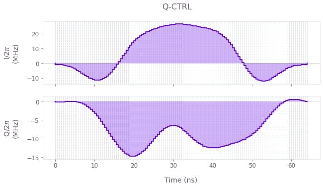

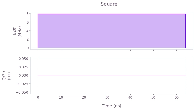
png-1

png-2

The control plots represent the $I(t)$ and $Q(t)$ components of the control pulses for: Boulder Opal optimizations (top) and the primitive control (bottom). Note that the robust pulse obtained is mostly symmetrical. If desired, time-symmetrical pulses can be enforced within the optimization.

Simulated time evolution of the driven qubit

Another useful way to characterize the pulses is to use the Boulder Opal simulation tool to obtain the time evolution of the system. This way one can observe the effect of arbitrary pulses on the qubit dynamics and check if the pulses are performing the desired operation. The next two cells run the simulations, extract the results, and plot them.

# Boulder Opal simulations.
simulated_bloch = {}
gate_times = {}
for scheme_name, control in gate_schemes.items():
    simulated_bloch[scheme_name], gate_times[scheme_name] = simulation_coherent(
        control, 100
    )

Your task (action_id="1827925") has started.
Your task (action_id="1827925") has completed.
Your task (action_id="1827930") is queued.
Your task (action_id="1827930") has started.
Your task (action_id="1827930") has completed.

# Plot results.
fig, axs = plt.subplots(1, len(gate_schemes.keys()), figsize=(15, 5))
fig.suptitle(f"Time evolution under control pulses for qubit {qubit}", y=1.1)

for idx, scheme_name in enumerate(gate_schemes.keys()):
    ax = axs[idx]
    for meas_basis in bloch_basis:
        ax.plot(
            gate_times[scheme_name] / nano,
            simulated_bloch[scheme_name][meas_basis],
            ls=bloch_lines[meas_basis],
            label=f"{meas_basis}: simulation",
        )
    ax.set_title(scheme_name)
    ax.set_xlabel("Time (ns)")

axs[0].set_ylabel("Bloch components")
hs, ls = axs[0].get_legend_handles_labels()
fig.legend(handles=hs, labels=ls, loc="center", bbox_to_anchor=(0.5, 1.0), ncol=3)

plt.show()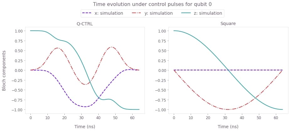

png-3

The simulated Bloch vector components $(x, y, z)$ of the state dynamics for the duration of the robust and primitive pulses.

Robustness characterization with filter functions and quasi-static scan

Filter functions provide a useful way to determine the sensitivity of pulses to different time varying noise mechanisms. The next cells generate filter functions for the Boulder Opal robust pulses and the primitive square pulse under dephasing noise.

sample_count = 4096
frequencies = np.logspace(-2, np.log10(omega_max), 2000)
filter_functions = {}

for scheme_name, control in gate_schemes.items():
    graph = bo.Graph()

    shift_I = graph.pwc(**control["I"]) * graph.pauli_matrix("X") / 2
    shift_Q = graph.pwc(**control["Q"]) * graph.pauli_matrix("Y") / 2

    duration = np.sum(shift_I.durations)
    drift = graph.constant_pwc_operator(
        duration=duration, operator=graph.pauli_matrix("Z")
    )

    graph.filter_function(
        control_hamiltonian=shift_I + shift_Q + drift,
        noise_operator=drift,
        frequencies=frequencies,
        sample_count=sample_count,
        name="filter_function",
    )

    result = bo.execute_graph(
        graph=graph, output_node_names="filter_function", execution_mode="EAGER"
    )

    filter_functions[scheme_name] = result["output"]["filter_function"]

Your task (action_id="1827944") is queued.
Your task (action_id="1827944") has started.
Your task (action_id="1827944") has completed.
Your task (action_id="1827959") has started.
Your task (action_id="1827959") has completed.

We next verify the pulse robustness against quasi-static noise by comparing the optimized $\pi$-pulses with the primitive pulse while detuning the drive frequency from the qubit frequency: $\Delta = \omega_\text{drive}-\omega_\text{qubit}$. This is tantamount to an effective dephasing term in the Hamiltonian, the strength and effect of which may be measured by scanning the detuning $\Delta$. The scan is calculated in the cell below.

gate_infidelity = {}
scan_array = np.linspace(-np.pi * mega, np.pi * mega, 21)
gate_infidelity["dephasing"] = {
    scheme_name: get_detuning_scan(scan_array, control)
    for scheme_name, control in gate_schemes.items()
}

Your task (action_id="1827969") is queued.
Your task (action_id="1827969") has started.
Your task (action_id="1827969") has completed.
Your task (action_id="1827977") is queued.
Your task (action_id="1827977") has started.
Your task (action_id="1827977") has completed.

Here's a plot of the filter functions and the detuning scan.

fig, axs = plt.subplots(1, 2, figsize=(15, 5))
fig.suptitle("Robustness verification", y=1.1)

ax = axs[0]
ax.set_xlabel("Frequency (Hz)")
ax.set_ylabel("Inverse power")
ax.set_title("Filter functions")
ax.set_xlim(np.min(frequencies), np.max(frequencies))
for scheme_name, _data in filter_functions.items():
    inverse_powers = _data["inverse_powers"]
    inverse_power_precisions = _data["uncertainties"]

    ax.loglog(
        frequencies, inverse_powers, "-", label=scheme_name, color=colors[scheme_name]
    )
    y_upper = inverse_powers + inverse_power_precisions
    y_lower = inverse_powers - inverse_power_precisions
    ax.fill_between(
        frequencies,
        y_lower,
        y_upper,
        hatch="||",
        alpha=0.35,
        facecolor="none",
        edgecolor=colors[scheme_name],
        linewidth=0.0,
    )

ax = axs[1]
ax.set_title("Robustness scan")
ax.set_ylabel("Ground state population")
ax.set_xlabel("Detuning (MHz)")
for name, infidelity in gate_infidelity["dephasing"].items():
    ax.plot(scan_array * 1e-6 / np.pi, infidelity, label=name, color=colors[name])

hs, ls = axs[0].get_legend_handles_labels()
fig.legend(handles=hs, labels=ls, loc="center", bbox_to_anchor=(0.5, 1.0), ncol=3)

plt.show()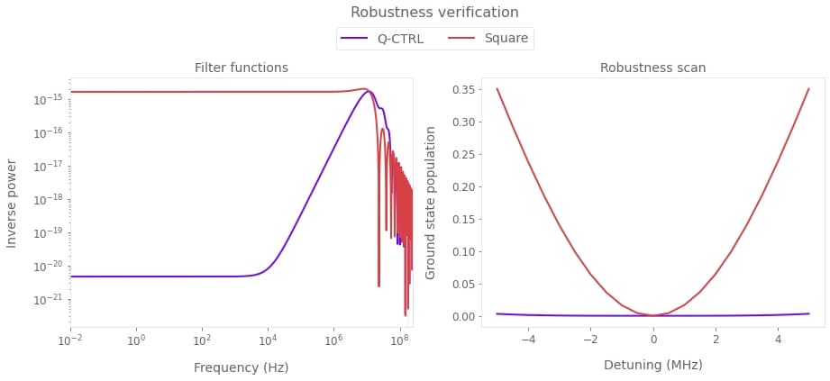

png-4

Left plot: Filter functions for the control pulses under dephasing noise. The hallmark of robustness is the significant drop of the filter function values at low frequencies. This feature is clearly demonstrated for the optimized Boulder Opal pulses. Right plot: Theoretical ground state population as a function of the detuning. The Boulder Opal solution shows flat behavior for a large range of detunings as compared to the primitive pulse, indicating robustness against dephasing.

Experimental time evolution of the driven qubit

We now compare the implementation and performance of the pulses discussed previously. A good test to check that the Boulder Opal pulses are being implemented properly in the IBM hardware is to compare the theoretical with the experimental time evolution of the qubit state. The next cell executes the different steps to obtain such a comparison:

Calibrate pulses for the specific IBM hardware,
Set up the schedules and run them on IBM-Q,
Extract and plot the resulting dynamics.

Note that here we use Rabi rate calibration data obtained previously for the ibmq_armonk device. To learn how to calibrate devices see the How to automate calibration of control hardware user guide.

# Calibrate pulses.
rabi_calibration_exp_I = load_variable(data_folder / "rabi_calibration_exp_I_demo")
pulse_amp_array = np.linspace(0.1, 1, 10)
pulse_amp_array = np.concatenate((-pulse_amp_array[::-1], pulse_amp_array))
f_amp_to_rabi = scipy.interpolate.interp1d(pulse_amp_array, rabi_calibration_exp_I)

amplitude_interpolated_list = np.linspace(-1, 1, 100)
rabi_interpolated_exp_I = f_amp_to_rabi(amplitude_interpolated_list)
f_rabi_to_amp = scipy.interpolate.interp1d(
    rabi_interpolated_exp_I, amplitude_interpolated_list
)

waveform = {}
for scheme_name, control in gate_schemes.items():
    I_values = control["I"]["values"] / (2 * np.pi)
    Q_values = control["Q"]["values"] / (2 * np.pi)
    A_I_values = np.repeat(f_rabi_to_amp(I_values), segment_scale[scheme_name])
    A_Q_values = np.repeat(f_rabi_to_amp(Q_values), segment_scale[scheme_name])
    waveform[scheme_name] = A_I_values + 1j * A_Q_values


# Create IBM schedules.
ibm_evolution_times = {}
times_int = {}
pulse_evolution_program = {}
time_min = 64
time_step = 64

for scheme_name in gate_schemes.keys():
    time_max = int(segment_scale[scheme_name] * number_of_segments[scheme_name])
    times_int[scheme_name] = np.arange(time_min, time_max + time_step, time_step)
    ibm_evolution_times[scheme_name] = times_int[scheme_name] * dt


if use_IBM is True:
    # Refresh backend.
    backend.properties(refresh=True)
    qubit_frequency_updated = backend.properties().qubit_property(qubit, "frequency")[0]

    for scheme_name in gate_schemes.keys():
        evolution_schedules = []
        for meas_basis in bloch_basis:
            for time_idx in times_int[scheme_name]:
                schedule = qs.pulse.Schedule(
                    name="Basis_%s_duration_%d" % (meas_basis, time_idx)
                )
                schedule += qs.pulse.Play(
                    qs.pulse.library.Waveform(waveform[scheme_name][:time_idx]),
                    drive_chan,
                )
                if meas_basis == "x":
                    schedule += inst_sched_map.get("u2", [0], P0=0.0, P1=np.pi)
                    schedule += measure_schedule << schedule.duration
                if meas_basis == "y":
                    schedule += inst_sched_map.get("u2", [0], P0=0.0, P1=np.pi / 2)
                    schedule += measure_schedule << schedule.duration
                if meas_basis == "z":
                    schedule += measure_schedule << schedule.duration
                evolution_schedules.append(schedule)

        pulse_evolution_program[scheme_name] = qs.compiler.assemble(
            evolution_schedules,
            backend=backend,
            meas_level=2,
            meas_return="single",
            shots=num_shots_per_point,
            schedule_los=[{drive_chan: qubit_frequency_updated}]
            * len(times_int[scheme_name])
            * 3,
        )

    if use_saved_data is False:
        # Run the jobs.
        evolution_exp_results = {}
        for scheme_name in gate_schemes.keys():
            job = backend.run(pulse_evolution_program[scheme_name])
            qs.tools.monitor.job_monitor(job)
            evolution_exp_results[scheme_name] = job.result(timeout=120)

        # Extract results.
        evolution_results_ibm = {}
        for scheme_name in gate_schemes.keys():
            evolution_basis = {}
            for meas_basis in bloch_basis:
                evolution_exp_data = np.zeros(len(times_int[scheme_name]))
                for idx, time_idx in enumerate(times_int[scheme_name]):
                    counts = evolution_exp_results[scheme_name].get_counts(
                        "Basis_%s_duration_%d" % (meas_basis, time_idx)
                    )
                    excited_pop = 0
                    for bits, count in counts.items():
                        excited_pop += count if bits[::-1][qubit] == "1" else 0
                    evolution_exp_data[idx] = excited_pop / num_shots_per_point
                evolution_basis[meas_basis] = evolution_exp_data
            evolution_results_ibm[scheme_name] = evolution_basis

        filename = data_folder / ("bloch_vectors_dephasing_" + timestr)
        save_variable(filename, evolution_results_ibm)
    else:
        filename = data_folder / "bloch_vectors_dephasing_demo"
        evolution_results_ibm = load_variable(filename)

else:
    filename = data_folder / "bloch_vectors_dephasing_demo"
    evolution_results_ibm = load_variable(filename)

# Plot results.
fig, axs = plt.subplots(1, len(gate_schemes.keys()), figsize=(15, 5))
fig.set_figheight(5)
fig.set_figwidth(16)
fig.suptitle(f"Time evolution under control pulses for qubit {qubit}", y=1.15)

for idx, scheme_name in enumerate(gate_schemes.keys()):
    ax = axs[idx]
    for meas_basis in bloch_basis:
        ax.plot(
            gate_times[scheme_name] / nano,
            simulated_bloch[scheme_name][meas_basis],
            ls=bloch_lines[meas_basis],
            color=bloch_colors[meas_basis],
            label=f"{meas_basis}: Q-CTRL simulation",
        )
        ax.plot(
            ibm_evolution_times[scheme_name] / nano,
            1 - 2 * evolution_results_ibm[scheme_name][meas_basis],
            bloch_markers[meas_basis],
            color=bloch_colors[meas_basis],
            label=f"{meas_basis}: IBM experiments",
        )
    ax.set_title(scheme_name)
    ax.set_xlabel("Time (ns)")

axs[0].set_ylabel("Bloch components")
hs, ls = axs[0].get_legend_handles_labels()
fig.legend(handles=hs, labels=ls, loc="center", bbox_to_anchor=(0.5, 1.02), ncol=3)

plt.show()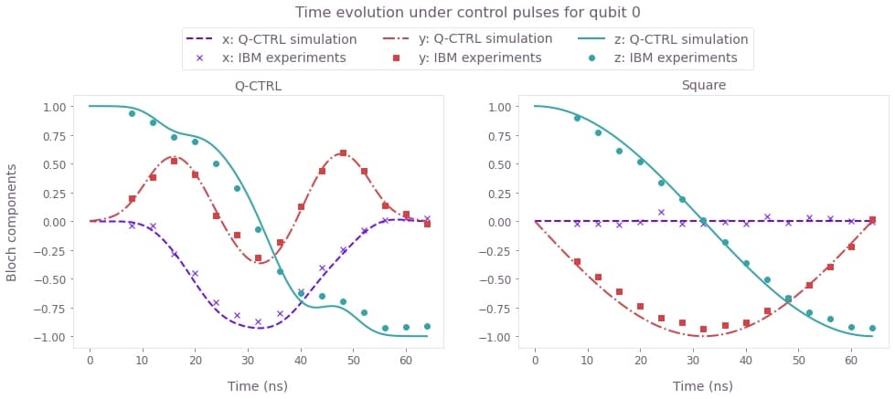

png-5

Comparison between the Bloch vector components (x, y, z) for the IBM experiments (symbols) and numerical simulation (lines). The smooth and band-limited Boulder Opal pulse waveform successfully implements the desired gate on the IBM hardware.

Experimental robustness verification with a quasi-static scan

To demonstrate the pulse robustness, we perform the experimental detuning scan, similar to what was done for the theoretical controls. As an extra comparison case, added to the scan here is the default X-gate for this IBM backend. The steps to achieve this are combined in the next execution cell, as follows:

Define detuning sweep interval,
Create schedules and run jobs on IBM-Q,
Extract results and produce robustness plot.

scheme_names.append("IBM default X-gate")
# Define detuning sweep interval.
detuning_array = np.linspace(
    qubit_frequency_updated - 1e6, qubit_frequency_updated + 1e6, 21
)
number_of_runs = 20
num_shots_per_point = 512

# Create schedules and run jobs.
if use_IBM is True and use_saved_data is False:
    drive_frequencies = [{drive_chan: freq} for freq in detuning_array]

    pi_experiment_results = {}
    for run in range(number_of_runs):
        for scheme_name in scheme_names:
            # Default IBM X-gate.
            if scheme_name == "IBM default X-gate":
                pi_schedule = qs.pulse.Schedule(name="IBM default X-gate")
                pi_schedule |= inst_sched_map.get(
                    "u3", [qubit], P0=np.pi, P1=0.0, P2=np.pi
                )
            else:
                pi_schedule = qs.pulse.Schedule(name=scheme_name)
                pi_schedule += qs.pulse.Play(
                    qs.pulse.library.Waveform(waveform[scheme_name]), drive_chan
                )
            pi_schedule += measure_schedule << pi_schedule.duration

            pi_experiment_ibm = qs.compiler.assemble(
                pi_schedule,
                backend=backend,
                meas_level=2,
                meas_return="single",
                shots=num_shots_per_point,
                schedule_los=drive_frequencies,
            )

            job = backend.run(pi_experiment_ibm)
            print(job.job_id())
            qs.tools.monitor.job_monitor(job)
            pi_experiment_results[scheme_name + str(run)] = job.result(timeout=120)

    # Extract results.
    detuning_sweep_results = {}
    for scheme_name in scheme_names:
        qctrl_sweep_values = np.zeros((number_of_runs, len(detuning_array)))
        for run in range(number_of_runs):
            i = 0
            for result in pi_experiment_results[scheme_name + str(run)].results:
                counts = result.data.counts["0x1"]
                excited_pop = counts / num_shots_per_point
                qctrl_sweep_values[run][i] = 1 - excited_pop
                i = i + 1
        detuning_sweep_results[scheme_name] = qctrl_sweep_values
    filename = data_folder / ("detuning_sweep_results_" + timestr)
    save_variable(filename, detuning_sweep_results)

else:
    filename = data_folder / "detuning_sweep_results_demo"
    detuning_sweep_results = load_variable(filename)

# Robustness plot.
fig, ax = plt.subplots(figsize=(10, 5))
for scheme_name, probability in detuning_sweep_results.items():
    ax.errorbar(
        detuning_array / mega - qubit_frequency_updated / mega,
        np.mean(probability, axis=0),
        yerr=np.std(probability, axis=0)
        / np.sqrt(len(detuning_sweep_results[scheme_name])),
        fmt="-o",
        markersize=5,
        capsize=3,
        label=f"{scheme_name} run on IBM-Q",
        color=colors[scheme_name],
    )
    if scheme_name != "IBM default X-gate":
        plt.plot(
            detuning_array / mega - qubit_frequency_updated / mega,
            gate_infidelity["dephasing"][scheme_name] + 0.075,
            linestyle="dashed",
            label=f"{scheme_name} simulation",
            color=colors[scheme_name],
        )

fig.suptitle("Detuning scan")
plt.xlabel("Detuning (MHz)")
plt.ylabel("Ground state population")
plt.legend()
plt.show()

png-6

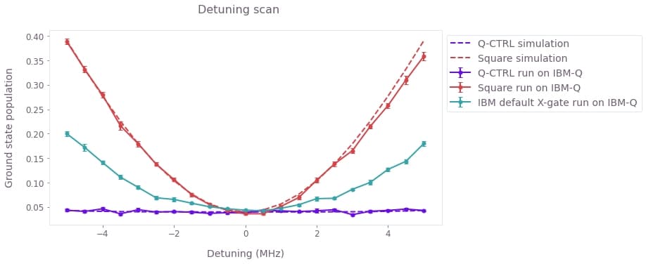
Experimental (symbols) and simulated (lines) ground state populations as a function of the detuning. The Boulder Opal control solution is mostly flat across the detuning scan, showing its robustness against dephasing noise as compared to the primitive square pulse as well as the default IBM X-gate. The theoretical curves have been shifted up by $0.075$ to account for measurement errors in the experimental data.

Other noise sources: Boulder Opal pulse robustness against control error

Besides robustness to dephasing, we next use Boulder Opal to design solutions that are robust against errors in the control amplitudes. The workflow is exactly as in the dephasing case:

Initialize Boulder Opal optimization parameters,
Run optimization and extract results,
Characterize robustness using filter functions,
Calibrate and implement pulses,
Verify robustness with an amplitude scan.

Creating pulses robust to control amplitude errors

The next cell contains all Boulder Opal commands to generate pulses for the control scenario defined previously. The only difference to the dephasing case is that the noise_operators are now time-varying terms of the control Hamiltonian.

number_of_segments = 256
number_of_optimization_variables = 64
segment_scale = 10
duration_int = number_of_segments * segment_scale
duration = duration_int * dt
cutoff_frequency = omega_max * 2.0
scheme_names = []

if use_saved_data is False:
    robust_amplitude_controls = {}

    graph = bo.Graph()

    # Create I & Q variables.
    I_values = graph.optimization_variable(
        count=number_of_optimization_variables, lower_bound=-I_max, upper_bound=I_max
    )
    Q_values = graph.optimization_variable(
        count=number_of_optimization_variables, lower_bound=-Q_max, upper_bound=Q_max
    )

    # Anchor ends to zero with amplitude rise/fall envelope.
    time_points = np.linspace(-1.0, 1.0, number_of_optimization_variables + 2)[1:-1]
    envelope_function = 1.0 - np.abs(time_points)
    I_values = I_values * envelope_function
    Q_values = Q_values * envelope_function

    # Create I & Q signals.
    I_signal = graph.pwc_signal(values=I_values, duration=duration)
    Q_signal = graph.pwc_signal(values=Q_values, duration=duration)

    # Apply the sinc filter and re-discretize signals.
    I_signal = graph.filter_and_resample_pwc(
        pwc=I_signal,
        kernel=graph.sinc_convolution_kernel(cutoff_frequency),
        segment_count=number_of_segments,
        name="I",
    )
    Q_signal = graph.filter_and_resample_pwc(
        pwc=Q_signal,
        kernel=graph.sinc_convolution_kernel(cutoff_frequency),
        segment_count=number_of_segments,
        name="Q",
    )

    # Create Hamiltonian control terms.
    I_term = I_signal * graph.pauli_matrix("X") / 2.0
    Q_term = Q_signal * graph.pauli_matrix("Y") / 2.0

    control_hamiltonian = I_term + Q_term

    # Create dephasing noise term.
    amplitude = control_hamiltonian

    # Create infidelity.
    infidelity = graph.infidelity_pwc(
        hamiltonian=control_hamiltonian,
        target=graph.target(X_gate),
        noise_operators=[amplitude],
        name="infidelity",
    )

    # Calculate optimization.
    result = bo.run_optimization(
        graph=graph,
        cost_node_name="infidelity",
        output_node_names=["I", "Q"],
        optimization_count=7,
    )

    print(f"Cost: {result['cost']}")

    robust_amplitude_controls["Q-CTRL"] = result["output"]

    filename = data_folder / ("robust_amplitude_controls_" + timestr)
    save_variable(filename, robust_amplitude_controls)
else:
    filename = data_folder / "robust_amplitude_controls_demo"
    robust_amplitude_controls = load_variable(filename)
scheme_names.append("Q-CTRL")

# Create square pulse.
square_pulse_value = np.array([rabi_rotation / duration])
square_sequence = {
    "I": {"durations": np.array([duration]), "values": square_pulse_value},
    "Q": {"durations": np.array([duration]), "values": np.zeros(1)},
}
scheme_names.append("Square")

# Combine all pulses into a single dictionary.
gate_schemes = {**robust_amplitude_controls, **{"Square": square_sequence}}

# Add IBM default X-gate.
scheme_names.append("IBM default X-gate")

for scheme_name, gate in gate_schemes.items():
    qv.plot_controls(gate)
    plt.suptitle(scheme_name)
    plt.show()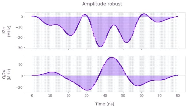

png-7

png-8

$I(t)$ and $Q(t)$ components of the control pulses for the optimized (top) and primitive (bottom) controls. Note that the duration of the pulses has increased. This is to enable testing of the robustness of the pulses later, by scanning over a large range of control amplitude errors. Therefore using longer pulses (and lower Rabi rates) will help to always stay within the maximum Rabi rate bounds given by the backend.

Time evolution of the driven qubit: simulations and experiment

As for the amplitude robust pulses, we calibrate the control-error-robust pulses using the interpolation obtained previously and run them on the IBM machine to compare the theoretical and experimental time evolution of the qubit state under no added noise. The cell below combines the following steps:

Pulse calibration,
Set up IBM schedules,
Run jobs on IBM-Q and extract results,
Run Boulder Opal simulations,
Plot results.

# Pulse calibration.
waveform = {}
for scheme_name, control in gate_schemes.items():
    I_values = control["I"]["values"] / (2 * np.pi)
    Q_values = control["Q"]["values"] / (2 * np.pi)
    if scheme_name == "Square":
        A_I_values = np.repeat(
            f_rabi_to_amp(I_values), segment_scale * number_of_segments
        )
        A_Q_values = np.repeat(
            f_rabi_to_amp(Q_values), segment_scale * number_of_segments
        )
    else:
        A_I_values = np.repeat(f_rabi_to_amp(I_values), segment_scale)
        A_Q_values = np.repeat(f_rabi_to_amp(Q_values), segment_scale)
    waveform[scheme_name] = A_I_values + 1j * A_Q_values

# Create IBM schedules.
time_min = 64
time_max = duration_int
time_step = 128
num_shots_per_point = 2048
times_int = np.arange(time_min, time_max + time_step, time_step)
ibm_evolution_times = times_int * dt
num_time_points = len(times_int)

if use_IBM is True:
    for scheme_name in gate_schemes.keys():
        evolution_schedules = []
        for meas_basis in bloch_basis:
            for time_idx in times_int:
                schedule = qs.pulse.Schedule(
                    name="Basis_%s_duration_%d" % (meas_basis, time_idx)
                )
                schedule += qs.pulse.Play(
                    qs.pulse.library.Waveform(waveform[scheme_name][:time_idx]),
                    drive_chan,
                )
                if meas_basis == "x":
                    schedule += inst_sched_map.get("u2", [0], P0=0.0, P1=np.pi)
                    schedule += measure_schedule << schedule.duration
                if meas_basis == "y":
                    schedule += inst_sched_map.get("u2", [0], P0=0.0, P1=np.pi / 2)
                    schedule += measure_schedule << schedule.duration
                if meas_basis == "z":
                    schedule += measure_schedule << schedule.duration
                evolution_schedules.append(schedule)

        pulse_evolution_program[scheme_name] = qs.compiler.assemble(
            evolution_schedules,
            backend=backend,
            meas_level=2,
            meas_return="single",
            shots=num_shots_per_point,
            schedule_los=[{drive_chan: qubit_frequency_updated}] * len(times_int) * 3,
        )

    if use_saved_data is False:
        evolution_exp_results = {}
        for scheme_name in gate_schemes.keys():
            job = backend.run(pulse_evolution_program[scheme_name])
            qs.tools.monitor.job_monitor(job)
            evolution_exp_results[scheme_name] = job.result(timeout=120)

        # Extract results.
        evolution_results_ibm = {}
        for scheme_name in gate_schemes.keys():
            evolution_basis = {}
            for meas_basis in bloch_basis:
                evolution_exp_data = np.zeros(len(times_int))
                for idx, time_idx in enumerate(times_int):
                    counts = evolution_exp_results[scheme_name].get_counts(
                        "Basis_%s_duration_%d" % (meas_basis, time_idx)
                    )
                    excited_pop = 0
                    for bits, count in counts.items():
                        excited_pop += count if bits[::-1][qubit] == "1" else 0
                    evolution_exp_data[idx] = excited_pop / num_shots_per_point
                evolution_basis[meas_basis] = evolution_exp_data
            evolution_results_ibm[scheme_name] = evolution_basis

        filename = data_folder / ("bloch_vectors_amplitude_" + timestr)
        save_variable(filename, evolution_results_ibm)
    else:
        filename = data_folder / "bloch_vectors_amplitude_demo"
        evolution_results_ibm = load_variable(filename)
else:
    filename = data_folder / "bloch_vectors_amplitude_demo"
    evolution_results_ibm = load_variable(filename)

# Boulder Opal simulations.
simulated_bloch = {}
gate_times = {}
for scheme_name, control in gate_schemes.items():
    simulated_bloch[scheme_name], gate_times[scheme_name] = simulation_coherent(
        control, 100
    )

Your task (action_id="1827982") is queued.
Your task (action_id="1827982") has started.
Your task (action_id="1827982") has completed.
Your task (action_id="1827984") is queued.
Your task (action_id="1827984") has started.
Your task (action_id="1827984") has completed.

# Plot results.
fig, axs = plt.subplots(1, len(gate_schemes.keys()), figsize=(15, 5))
fig.suptitle(f"Time evolution under control pulses for qubit {qubit}", y=1.15)

for idx, scheme_name in enumerate(gate_schemes.keys()):
    ax = axs[idx]
    for meas_basis in bloch_basis:
        ax.plot(
            gate_times[scheme_name] / nano,
            simulated_bloch[scheme_name][meas_basis],
            ls=bloch_lines[meas_basis],
            color=bloch_colors[meas_basis],
            label=f"{meas_basis}: Q-CTRL simulation",
        )
        ax.plot(
            ibm_evolution_times / nano,
            1 - 2 * evolution_results_ibm[scheme_name][meas_basis],
            bloch_markers[meas_basis],
            color=bloch_colors[meas_basis],
            label=f"{meas_basis}: IBM experiments",
        )

    ax.set_title(scheme_name)
    ax.set_xlabel("Time (ns)")

axs[0].set_ylabel("Bloch components")
hs, ls = axs[0].get_legend_handles_labels()
fig.legend(handles=hs, labels=ls, loc="center", bbox_to_anchor=(0.5, 1.02), ncol=3)

plt.show()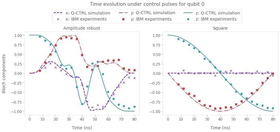

png-9

Time evolution of the Bloch vector components (x, y, z) for simulations (lines) and experimental runs (symbols) under the control-robust pulses.

Experimental robustness verification with a quasi-static scan and filter functions

We again assess the sensitivity of the pulses to the noise using filter functions and quasi-static noise-susceptibility scans. The only difference here is the change in the noise process, which is achieved by replacing the dephasing term by noise on the controls. The filter functions calculated in the cell below use noise in the $I$ and $Q$ components of the controls.

sample_count = 4096
frequencies = np.logspace(-2, np.log10(omega_max), 2000)
filter_functions = {}

for scheme_name, control in gate_schemes.items():
    graph = bo.Graph()

    shift_I = graph.pwc(**control["I"]) * graph.pauli_matrix("X") / 2
    shift_Q = graph.pwc(**control["Q"]) * graph.pauli_matrix("Y") / 2

    control_hamiltonian = shift_I + shift_Q

    graph.filter_function(
        control_hamiltonian=control_hamiltonian,
        noise_operator=control_hamiltonian,
        frequencies=frequencies,
        sample_count=sample_count,
        name="filter_function",
    )

    result = bo.execute_graph(
        graph=graph, output_node_names="filter_function", execution_mode="EAGER"
    )

    filter_functions[scheme_name] = result["output"]["filter_function"]

Your task (action_id="1827987") is queued.
Your task (action_id="1827987") has started.
Your task (action_id="1827987") has completed.
Your task (action_id="1827991") has started.
Your task (action_id="1827991") has completed.

We also demonstrate robustness by performing a quasi-static control-error scan, both numerically and experimentally. The steps follow the same structure as in the dephasing case and are combined in the next cell:

Define control error range,
Create schedules and run them on IBM-Q,
Create Boulder Opal theoretical control error scan.

scheme_names = ["Q-CTRL", "Square", "IBM default X-gate"]
# Define control amplitude error range.
amp_error = 0.25
amp_scalings = np.linspace(1 - amp_error, amp_error + 1, 21)

# Define schedules and run jobs.
if use_IBM is True and use_saved_data is False:
    IBM_default_X_gate_schedule = inst_sched_map.get(
        "u3", [qubit], P0=np.pi, P1=0.0, P2=np.pi
    )
    pi_experiment_results = {}
    for run in range(number_of_runs):
        for scheme_name in scheme_names:
            pi_schedule = []
            for amp_scaling in amp_scalings:
                if scheme_name == "IBM default X-gate":
                    this_schedule = qs.pulse.Schedule(name=scheme_name)
                    for idx, inst in enumerate(
                        IBM_default_X_gate_schedule.instructions
                    ):
                        if inst[1].name is None:
                            this_schedule |= qs.pulse.Schedule(inst)
                        else:  # if "X90" in inst[1].name:
                            Ival = np.real(inst[1].instructions[0][1].pulse.samples)
                            Qval = np.imag(inst[1].instructions[0][1].pulse.samples)
                            phasors = Ival + 1j * Qval
                            this_schedule |= (
                                qs.pulse.Play(
                                    qs.pulse.library.Waveform(phasors * amp_scaling),
                                    inst[1].channels[0],
                                )
                                << this_schedule.duration
                            )
                    this_schedule += measure_schedule << this_schedule.duration
                    pi_schedule.append(this_schedule)
                else:
                    this_schedule = qs.pulse.Schedule(name=scheme_name)
                    this_schedule += (
                        qs.pulse.Play(
                            qs.pulse.library.Waveform(
                                waveform[scheme_name] * amp_scaling
                            ),
                            drive_chan,
                        )
                        << 1
                    )
                    this_schedule += measure_schedule << duration_int
                    pi_schedule.append(this_schedule)

            num_shots_per_point = 512

            pi_experiment_ibm = qs.compiler.assemble(
                pi_schedule,
                backend=backend,
                meas_level=2,
                meas_return="single",
                shots=num_shots_per_point,
                schedule_los=[{drive_chan: qubit_frequency_updated}]
                * len(amp_scalings),
            )
            job = backend.run(pi_experiment_ibm)
            print(job.job_id())
            qs.tools.monitor.job_monitor(job)
            pi_experiment_results[scheme_name + str(run)] = job.result(timeout=120)

    # Extracting results.
    amplitude_sweep_results = {}
    for scheme_name in scheme_names:
        qctrl_sweep_values = np.zeros((number_of_runs, len(amp_scalings)))
        for run in range(number_of_runs):
            i = 0
            for result in pi_experiment_results[scheme_name + str(run)].results:
                counts = result.data.counts["0x1"]
                excited_pop = counts / num_shots_per_point
                qctrl_sweep_values[run][i] = 1 - excited_pop
                i = i + 1
        amplitude_sweep_results[scheme_name] = qctrl_sweep_values
    filename = data_folder / ("amplitude_sweep_results_" + timestr)
    save_variable(filename, amplitude_sweep_results)
else:
    filename = data_folder / "amplitude_sweep_results_demo"
    amplitude_sweep_results = load_variable(filename)

# Boulder Opal control amplitude scan.
gate_infidelity = {}
amplitude_array = np.linspace(-0.25, 0.25, 21)
gate_infidelity["amplitude"] = {
    scheme_name: get_amplitude_scan(amplitude_array, control)
    for scheme_name, control in gate_schemes.items()
}

Your task (action_id="1827992") has completed.
Your task (action_id="1827994") is queued.
Your task (action_id="1827994") has completed.

Next, we plot the numerical filter functions and the control error scan.

fig, axs = plt.subplots(1, 2, figsize=(15, 5))
fig.suptitle("Robustness verification", y=1)

ax = axs[0]
ax.set_xlabel("Frequency (Hz)")
ax.set_ylabel("Inverse power")
ax.set_title("Filter functions")
ax.set_xlim(np.min(frequencies), np.max(frequencies))

for scheme_name, _data in filter_functions.items():
    inverse_powers = _data["inverse_powers"]
    inverse_power_precisions = _data["uncertainties"]

    ax.loglog(
        frequencies, inverse_powers, "-", label=scheme_name, color=colors[scheme_name]
    )
    y_upper = inverse_powers + inverse_power_precisions
    y_lower = inverse_powers - inverse_power_precisions
    ax.fill_between(
        frequencies,
        y_lower,
        y_upper,
        hatch="||",
        alpha=0.35,
        facecolor="none",
        edgecolor=colors[scheme_name],
        linewidth=0.0,
    )
ax.legend()

ax = axs[1]
ax.set_title("Robustness scan")
ax.set_ylabel("Ground state population")
ax.set_xlabel("Control amplitude error")
for scheme_name, probability in amplitude_sweep_results.items():
    ax.errorbar(
        amp_scalings - 1,
        np.mean(probability, axis=0),
        yerr=np.std(probability, axis=0)
        / np.sqrt(len(amplitude_sweep_results[scheme_name])),
        fmt="-o",
        capsize=5,
        label=f"{scheme_name} run on IBM-Q",
        color=colors[scheme_name],
    )
    if scheme_name != "IBM default X-gate":
        ax.plot(
            amp_scalings - 1,
            gate_infidelity["amplitude"][scheme_name] + 0.071,
            linestyle="dashed",
            label=f"{scheme_name} simulation",
            color=colors[scheme_name],
        )
ax.legend()
plt.show()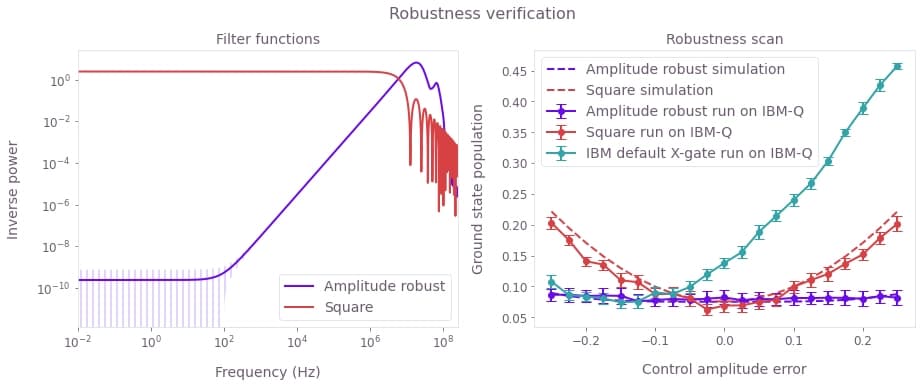

png-10

Left plot: Filter functions for the control pulses under control noise in the $I$ component. Again, robustness is clearly demonstrated for the optimized Boulder Opal pulses. Right plot: Experimental (symbols) and simulated (lines) ground state populations as a function of the error in the control amplitude (note that the control amplitudes vary between -1 and 1). The Boulder Opal control solution is robust, with a flat response for a large range of control errors as compared to the primitive pulse. The theoretical curves have been shifted up by $0.071$ to account for measurement errors in the experimental data.