How to optimize controls using gradient-free optimization

In addition to a highly-flexible optimization engine for general-purpose gradient-based optimization, Boulder Opal also features a gradient-free optimizer which can be directly applied to model-based control optimization for arbitrary-dimensional quantum systems.

The gradient-free optimizer is exposed by the boulderopal.run_gradient_free_optimization function, which works similarly to boulderopal.run_optimization, with most of the parameters overlapping between the two functions. While the gradient-based optimization is more likely to find better results quicker, the gradient-free optimizer is useful in cases where the gradient is either very costly to compute or inaccessible (for example if the graph includes a node that does not allow gradients). Also since the gradient is not computed, the memory requirements for the gradient-free optimizer are much lower.

The optimization engine from Boulder Opal allows the user to express their system Hamiltonians as almost-arbitrary functions of the controllable parameters. The underlying structure of this map is a graph, which defines the cost function and can be efficiently evaluated. The resulting optimized controls thus achieve the desired objectives within the constraints imposed by the user-defined Hamiltonian structure.

The example in this user guide illustrates how to optimize multiple controls under different constraints in a single system using the gradient-free optimizer.

Summary workflow

1. Define the computational graph

The Boulder Opal optimization engine expresses all optimization problems as data flow graphs, which you can create by initializing a boulderopal.Graph class. The methods of the graph object allow you to represent the mathematical structure of the problem that you want to solve.

For an optimization, a typical workflow is to:

• Create "signals", or scalar-valued functions of time, which typically represent control pulses.
• Create "operators", or matrix-valued functions of time, by modulating constant operators by signals. These typically represent terms of a Hamiltonian.
• Combine the operators into a single Hamiltonian operator.
• Calculate the optimization cost function (typically an infidelity) from the Hamiltonian.

2. Run graph-based gradient-free optimization

You can calculate an optimization from an input graph using the boulderopal.run_gradient_free_optimization function. Provide the name of the node of the graph that represents the cost, and this function will return the optimized value of the output nodes that you requested. Unlike boulderopal.run_optimization, which uses the gradient and halts when it has converged to a minimum, boulderopal.run_gradient_free_optimization cannot rely on such convergence criteria. Instead, the function stops after performing iteration_count iterations (which defaults to 100), unless the cost reaches a value below target_cost (if you provide one).

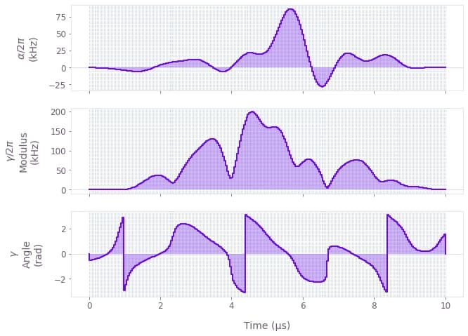
Example: Optimal control of a single qubit

This example shows how to optimize a Hamiltonian with multiple controls. Specifically, consider a single-qubit system represented by the following Hamiltonian:

\begin{equation}H(t) = \frac{\nu}{2} \sigma_{z} + \frac{1}{2}\left[\gamma(t)\sigma_{-} + \gamma^*(t)\sigma_{+}\right] + \frac{\alpha(t)}{2} \sigma_{z} ,\end{equation}

where $\nu$ is the qubit detuning, $\gamma(t)$ and $\alpha(t)$ are, respectively, complex and real time-dependent pulses, $\sigma_{\pm}$ are the qubit ladder operators, and $\sigma_{z}$ is the Pauli-Z operator.

The functions of time $\gamma(t)$ and $\alpha(t)$ are not predetermined, and instead are optimized by Boulder Opal in order to achieve the target operation, which in this case is a Y-gate.

import numpy as np
import qctrlvisualizer as qv
import boulderopal as bo

# Define physical constants.
nu = 2 * np.pi * 5e5  # rad/s
gamma_max = 2 * np.pi * 3e5  # rad/s
alpha_max = 2 * np.pi * 1e5  # rad/s
cutoff_frequency = 5e6  # Hz
segment_count = 50
duration = 10e-6  # s

graph = bo.Graph()

# Create the time-independent detuning term.
detuning = nu * graph.pauli_matrix("Z") / 2

# Add a cosine envelope to the signals, to ensure
# they go to zero at the beginning and end of pulse.
cos_envelope = graph.signals.cosine_pulse_pwc(
    duration=duration, segment_count=256, amplitude=1.0
)

# Create an optimizable complex-valued piecewise-constant (PWC) signal.
rough_gamma = graph.complex_optimizable_pwc_signal(
    segment_count=segment_count, maximum=gamma_max, duration=duration
)
# Smooth the signal.
gamma = graph.filter_and_resample_pwc(
    pwc=rough_gamma,
    segment_count=256,
    kernel=graph.sinc_convolution_kernel(cutoff_frequency),
)
gamma = gamma * cos_envelope
gamma.name = r"$\gamma$"

# Create a PWC operator representing the drive term.
drive = graph.hermitian_part(gamma * graph.pauli_matrix("M"))

# Create an optimizable real-valued PWC signal.
rough_alpha = graph.real_optimizable_pwc_signal(
    segment_count=segment_count,
    minimum=-alpha_max,
    maximum=alpha_max,
    duration=duration,
)
# Smooth the signal.
alpha = graph.filter_and_resample_pwc(
    pwc=rough_alpha,
    segment_count=256,
    kernel=graph.sinc_convolution_kernel(cutoff_frequency),
)
alpha = alpha * cos_envelope
alpha.name = r"$\alpha$"

# Create a PWC operator representing the clock shift term.
shift = alpha * cos_envelope * graph.pauli_matrix("Z") / 2

# Define the total Hamiltonian and the target operation.
hamiltonian = detuning + drive + shift
target = graph.target(graph.pauli_matrix("Y"))

# Create the infidelity.
infidelity = graph.infidelity_pwc(hamiltonian, target, name="infidelity")

# Run the optimization.
result = bo.run_gradient_free_optimization(
    graph=graph,
    cost_node_name="infidelity",
    output_node_names=[r"$\alpha$", r"$\gamma$"],
    target_cost=5e-3,
)
print(f"Optimized cost:\t{result['cost']:.3e}")

# Plot the optimized controls.
qv.plot_controls(result["output"])

Your task (action_id="1824881") is queued.
Your task (action_id="1824881") has started.
Your task (action_id="1824881") has completed.
Optimized cost:	5.715e-03