How to optimize controls in arbitrary quantum systems using graphs

Boulder Opal provides a highly-flexible optimization engine for general-purpose gradient-based optimization. It can be directly applied to model-based control optimization for arbitrary-dimensional quantum systems.

The optimization engine from Boulder Opal allows the user to express their system Hamiltonians as almost-arbitrary functions of the controllable parameters. The underlying structure of this map is a graph, which defines the cost function and can be efficiently evaluated and differentiated. The resulting optimized controls thus achieve the desired objectives within the constraints imposed by the user-defined Hamiltonian structure.

The example in this user guide illustrates how to optimize multiple controls under different constraints in a single system. For a step-by-step description of how to create a robust optimization with multiple controls, see our tutorial Design robust single-qubit gates using computational graphs.

Summary workflow

1. Define the computational graph

The Boulder Opal optimization engine expresses all optimization problems as data flow graphs, which you can create a graph object by initializing the boulderopal.Graph class. The methods of the graph object allow you to represent the mathematical structure of the problem that you want to solve.

For an optimization, a typical workflow is to:

• Create "signals", or scalar-valued functions of time, which typically represent control pulses.
• Create "operators", or matrix-valued functions of time, by modulating constant operators by signals. These typically represent terms of a Hamiltonian.
• Combine the operators into a single Hamiltonian operator.
• Calculate the optimization cost function (typically an infidelity) from the Hamiltonian.

2. Execute graph-based optimization

You can calculate an optimization from an input graph using the boulderopal.run_optimization function. Provide the name of the node of the graph that represents the cost, and this function will return the optimized value of the output nodes that you requested.

Example: Optimal control of a single qubit

This example shows how to optimize a Hamiltonian with multiple controls. Specifically, consider a single-qubit system represented by the following Hamiltonian:

\begin{align} H(t) &= \frac{\nu}{2} \sigma_{z} + \frac{1}{2}\left[\gamma(t)\sigma_{-} + \gamma^*(t)\sigma_{+}\right] + \frac{\alpha(t)}{2} \sigma_{z} , \end{align}

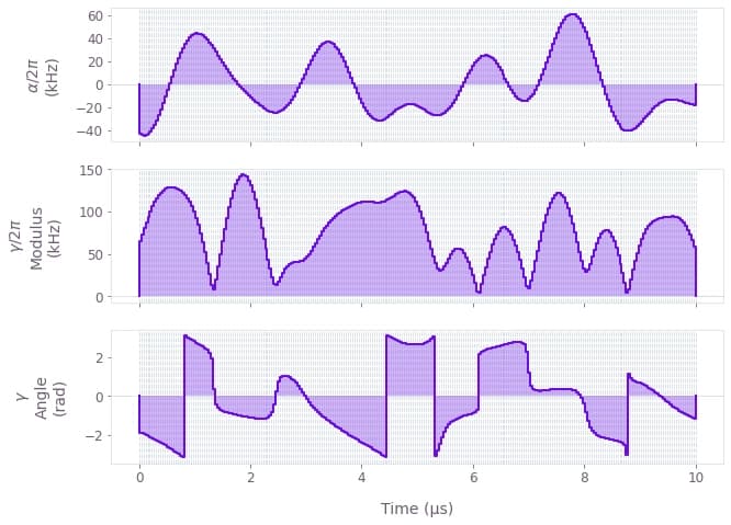
where $\nu$ is the qubit detuning, $\gamma(t)$ and $\alpha(t)$ are, respectively, complex and real time-dependent pulses, $\sigma_{\pm}$ are the qubit ladder operators, and $\sigma_{z}$ is the Pauli-Z operator.

The functions of time $\gamma(t)$ and $\alpha(t)$ are not predetermined, and instead are optimized by Boulder Opal in order to achieve the target operation, which in this case is a Y-gate.

import numpy as np
import qctrlvisualizer as qv
import boulderopal as bo

# Define physical constants.
nu = 2 * np.pi * 5e5  # rad/s
gamma_max = 2 * np.pi * 3e5  # rad/s
alpha_max = 2 * np.pi * 1e5  # rad/s
cutoff_frequency = 5e6  # Hz
segment_count = 50
duration = 10e-6  # s

# Create the graph describing the system.
graph = bo.Graph()

# Create the time-independent detuning term.
detuning = nu * graph.pauli_matrix("Z") / 2

# Create a optimizable complex-valued piecewise-constant (PWC) signal.
rough_gamma = graph.complex_optimizable_pwc_signal(
    segment_count=segment_count, maximum=gamma_max, duration=duration
)
# Smooth the signal.
gamma = graph.filter_and_resample_pwc(
    pwc=rough_gamma,
    segment_count=256,
    kernel=graph.sinc_convolution_kernel(cutoff_frequency),
    name=r"$\gamma$",
)

# Create a PWC operator representing the drive term.
drive = graph.hermitian_part(gamma * graph.pauli_matrix("M"))

# Create an optimizable real-valued PWC signal.
rough_alpha = graph.real_optimizable_pwc_signal(
    segment_count=segment_count,
    minimum=-alpha_max,
    maximum=alpha_max,
    duration=duration,
)
# Smooth the signal.
alpha = graph.filter_and_resample_pwc(
    pwc=rough_alpha,
    segment_count=256,
    kernel=graph.sinc_convolution_kernel(cutoff_frequency),
    name=r"$\alpha$",
)
# Create a PWC operator representing the clock shift term.
shift = alpha * graph.pauli_matrix("Z") / 2

# Define the total Hamiltonian and the target operation.
hamiltonian = detuning + drive + shift
target = graph.target(graph.pauli_matrix("Y"))

# Create the infidelity.
infidelity = graph.infidelity_pwc(hamiltonian, target, name="infidelity")

# Run the optimization.
result = bo.run_optimization(
    graph=graph,
    cost_node_name="infidelity",
    output_node_names=[r"$\alpha$", r"$\gamma$"],
    optimization_count=4,
)
print(f"Optimized cost:\t{result['cost']:.3e}")

# Plot the optimized controls.
qv.plot_controls(result["output"])

Your task (action_id="1828657") has started.
Your task (action_id="1828657") has completed.
Optimized cost:	5.129e-13