Leverage predefined signals in graphs

The controls used in quantum devices often take the form of signals that are variations over predefined shapes. For example, you can choose to embed your signal in a Gaussian envelope, to make sure that your controls evolve gradually from zero to their peak, and then back to zero again. Boulder Opal equips you predefined signal functions, to make it easier for you to create signals according to certain standardized shapes. With them, you only need to provide the minimum required number of parameters that characterize their shapes to create your signals.

In this topic, we discuss signals that belong in graphs and can therefore be used in optimization and simulation. We will explain how you can use this graph-based signal library and show examples of the signals that you can generate with it.

Note that Boulder Opal also has a library of signals independent of the graph framework. These are suitable to be used with closed-loop optimization, because they can easily be exported to external quantum computing backends such as Qiskit, Pyquil, and QUA. You can learn more about it in this topic.

Signals library

Signals that are represented as graph nodes can be used as normal controls in a system that you model using the graph representation. You can use these nodes when you want to perform an optimization using boulderopal.run_optimization or boulderopal.run_stochastic_optimization, or a simulation using boulderopal.execute_graph.

You can find these signals in the graph.signals namespace of the Graph object in two types of forms: piecewise constant (PWC) signals, which are discretized into segments of constant value, and sampleable tensor-valued function (STF) signals, which are smooth in their shape. These two object types are described and compared in the topic Working with time-dependent functions in Boulder Opal. Most of the signals are available in both PWC and STF output formats, except for those signals that contain discontinuities, which are only available in PWC format. The functions for the two types of signals are distinguished by their suffixes, which are either _pwc or _stf. For most applications, a signal in PWC format is sufficient.

The signals in both formats are usually quite similar, with the inevitable difference that PWC signals are discretized into segments of constant value. For this reason, PWC signals require the parameters segment_count and duration, which are not present in STF signals. The higher the number of segments that you provide in this parameter, the more finely grained the signal will be discretized, and the closer it will be to its STF equivalent.

Some PWC signals contain parts that are constant, such as the flat part of a flat-top pulse. In that case, the relevant PWC signal node, for instance, graph.signals.gaussian_pulse_pwc, accepts a segmentation parameter. With this, you can choose between a uniform segmentation, where the PWC segments are uniformly distributed along the signal's duration, or a minimal segmentation, where the constant parts of the PWC function are represented with a minimal number of segments, reserving most of the segments for the non-constant parts. A uniform segmentation is preferred when combining different signals, while a minimal segmentation leads to a more efficient sampling of the non-constant parts.

Note that many of the parameters that you can pass to the graph signal functions can be Tensors, which means that they can be optimized. For example, if you want to find out what is the width and amplitude of a Gaussian pulse to best perform a certain operation, you can pass these two parameters as optimizable tensors to the graph.signals.gaussian_pulse_pwc function and then run an optimization, using the infidelity of the gate as the cost function. The Boulder Opal optimizer will then tell you which values of the parameters minimize the infidelity.

To learn more about graph signals, please read their reference documentation.

Signal types

The libraries of signals have similar kinds of signals shared among them. In the rest of this topic, we present an overview of the main types:

• Pulses: controls that go from zero to a peak, and then back to zero.
• Oscillations: controls that consist of oscillating functions that might have multiple peaks.
• Ramps: controls that monotonically vary from an initial value to a final value.

Pulses

These are signals that go (either asymptotically or strictly) from zero to a peak, and then back to zero. The Boulder Opal libraries of signals include these pulse types:

• Gaussian pulses (graph.signals.gaussian_pulse_pwc and graph.signals.gaussian_pulse_stf).
• Hyperbolic secant pulses (graph.signals.sech_pulse_pwc and graph.signals.sech_pulse_stf).
• Cosine pulses (graph.signals.cosine_pulse_pwc).

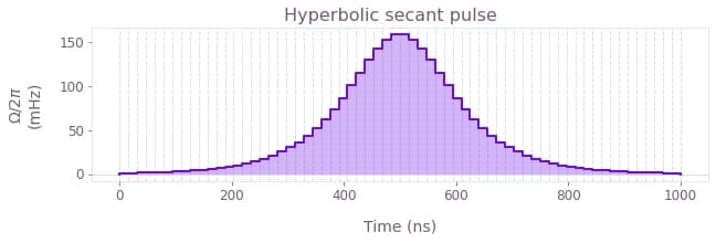
The next figure illustrates what a hyperbolic secant pulse created with the Boulder Opal library of signals looks like.

A particular case of these pulses is the square pulse, which has a finite value equal to its amplitude during a specified length of time, and is zero for all the rest of the time. Due to this discontinuity, the square pulse can't be created as an STF. To learn more about square pulses for Boulder Opal, see the reference documentation for graph.signals.square_pulse_pwc.

Oscillations

It is possible to create pulses of many different shapes using superpositions of sines and cosines with different frequencies. In the Boulder Opal libraries of signals, these pulses can be found in the form of generic sinusoids or as a Hann series of squared sines with increasingly higher frequencies. To learn more about these oscillatory pulses, see the reference documentation for:

• Sinusoids (graph.signals.sinusoid_pwc and graph.signals.sinusoid_stf).
• Hann series (graph.signals.hann_series_pwc and graph.signals.hann_series_stf).

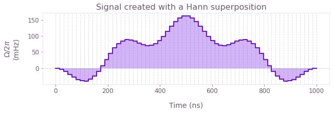
The Hann series in particular can be used as a basis for pulses that are zero at the extremities. The following plot shows an example of a PWC signal created with a Hann superposition.

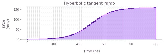
Ramps

Some signals of the signal library are continuously increasing or decreasing, instead of having a peak-like profile. These are called ramps, and you can learn more about them in the reference documentation for:

• Linear ramps (graph.signals.linear_ramp_pwc and graph.signals.linear_ramp_stf).

• Hyperbolic tangent ramps (graph.signals.tanh_ramp_pwc and graph.signals.tanh_ramp_stf).

You can also find usage examples of the library of signals in the user guide How to create analytical signals for simulation and optimization. For further information about it, take a look at the reference documentation for the signal library.