Working with time-dependent functions in Boulder Opal

Boulder Opal uses graphs to represent simulations and optimizations of quantum systems. The graph calculations can range from simple arithmetic to complex operations on high-dimensional quantum systems. Most Boulder Opal calculations involve time-dependent functions to represent, for instance, controls or dynamic Hamiltonians. This topic covers the different kinds of time-dependent functions in Boulder Opal graphs: what they are, and why we use them.

For a basic overview on how Boulder Opal uses computational graphs to represent systems and perform operations, you can read our Understanding graphs in Boulder Opal topic.

Time-dependent functions as graph nodes

Boulder Opal has two node types to represent time-dependent functions.

STFs are sampleable tensor-valued functions, a general representation of time-dependent functions. They are called "sampleable" as they can be sampled at arbitrary values of time. For instance, sampling the values of a continuous Hamiltonian at particular times to calculate its corresponding time-evolution operators.

On the other hand, PWCs represent piecewise-constant functions of time. Although they are less general than STFs, it is much easier to perform operations such as integration on PWCs, as they have constant values at different segments. Therefore, using PWCs when calculating the time evolution of a system is usually more efficient than using STFs.

In what follows, we will discuss how to create, manipulate, and export these two types in a Boulder Opal graph.

PWCs

A PWC represents a piecewise-constant (PWC) function. That is, the function takes discrete values $\{ \alpha_n \}$ at $N$ different segments, with durations $\{ \tau_n \}$. The segment durations can be different to each other, although it's common to have equally spaced segmentations. It is also convenient to define the total duration of the PWC, $T \equiv \sum_{n=1}^N \tau_n$.

We can write this type of function as: \begin{equation} \alpha(t) = \alpha_n \quad \mathrm{for} \quad t_n \leq t < t_{n+1} \, , \\ \end{equation} where $t_0 = 0$ and $t_n = t_{n-1} + \tau_n$. We can also assume that the function is 0 for $t < 0$ and $t > t_N = T$.

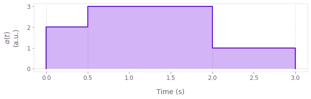
For example, the PWC function \begin{equation} \alpha(t) = \begin{cases} 2 \quad \mathrm{for} \quad 0 \leq t < 0.5 \\ 3 \quad \mathrm{for} \quad 0.5 \leq t < 2 \\ 1 \quad \mathrm{for} \quad 2 \leq t < 3 \\ \end{cases} \, , \end{equation} has three segments of durations 0.5, 1.5, and 1 seconds (a total duration of 0.5 + 1.5 + 1 = 3 seconds), and values 2, 3, and 1 (a.u.). It looks like this:

Creating PWCs

Boulder Opal graphs have a variety of operations to create PWC signals, depending on their characteristics. The most general operation is graph.pwc, creating a PWC from a Tensor (or array) of values. In some cases, however, other nodes are more convenient.

Signals

The function plotted above is a scalar-valued function, which we call a signal in Boulder Opal. Signals are often used for representing time-dependent coefficients in the Hamiltonian.

The operations graph.pwc_signal and graph.complex_pwc_signal create PWC signals, taking an array with the values at each segment and its total duration. These operations will create a uniform segmentation; the duration of each segment will be the total duration divided by the number of values that you provided. (If you want to create a signal with a non-uniform segmentation, you can use the more general graph.pwc node.)

Operators

You can also create matrix-valued functions, representing time-dependent operators such as Hamiltonians (or Hamiltonian terms).

In most cases, when creating a PWC operator, it has the form $H(t) = \alpha(t) A$, where $\alpha(t)$ is a signal and $A$ is a (constant) operator/matrix. In that case, you can create a node representing $H(t)$ by multiplying a PWC node representing $\alpha(t)$ by a Tensor (or NumPy array) representing $A$. That is equivalent to using the graph.pwc_operator operation.

Manipulating PWCs

We offer several graph operations for working with PWCs. These include nodes to create them, sample them, or manipulate them in the time dimension. Mathematical operations can also be directly applied to PWCs. For example you can calculate mathematical functions of a PWC, or use arithmetic operations between two PWCs. This allows you to create new time-dependent functions by manipulating a PWC or combining different ones. You can learn more about these operations in the Understanding graphs in Boulder Opal topic.

Note that you can also perform operations between a PWC and a tensor, where the tensor will be treated as a constant PWC, that is, a PWC with a single segment. If you want to operate with a constant batched PWC, you can use the operations graph.constant_pwc, graph.constant_pwc_operator to create a constant PWC.

Boulder Opal also includes operations to manipulate the behavior of PWCs in their time dimension: graph.symmetrize_pwc, graph.time_reverse_pwc, and graph.time_concatenate_pwc.

Extracting PWCs from a graph and plotting them

Similar to Tensors, you cannot directly know the values of PWC graph nodes, as their values have to first be extracted from the graph.

You can assign a name to a PWC by passing a name keyword argument to the operation creating it (or by directly assigning it to the PWCs name attribute). You can retrieve a PWC from a graph by adding its name to the output_node_names argument of, for example, boulderopal.execute_graph. The output dictionary in the calculation result will contain a key with the name of your node.

You can pass this output to the plot_controls function in the qctrlvisualizer package to obtain a plot of your function. You can see examples of this in our graphs and optimization tutorials.

Attributes of PWC nodes

PWC nodes have several attributes that you can access in order to get information about them.

• values: A Tensor containing the values of the function at each piecewise-constant segment. It has a shape of batch_shape + (segment_count,) + value_shape, where segment_count is the number of segments in the PWC function.

• durations: A NumPy array containing the segment durations.

• value_shape: A tuple indicating the shape of the values of the function. This would be () for a signal, and, for example, (4,4) for an operator.

• batch_shape: A tuple indicating the shape of the batch in the function, allowing you to efficiently perform multiple parallel computations. You can learn more about batching in the Batching and broadcasting in Boulder Opal topic.

You can access these attributes with the dot operation. For example, to get the durations of your PWC Hamiltonian, use hamiltonian.durations.

STFs

STFs are sampleable tensor-valued functions of time. They usually represent smooth functions, with or without an analytical form.

As we mentioned above, STFs can be sampled at different values of time. In most cases, the precision of a calculation with a continuous function will depend on how finely it is sampled. This is something one has to keep in mind when working with STFs and passing sampling times to the different evolution operations. PWCs do not suffer from this issue.

Creating STFs

There are two main ways to create an STF inside of a graph.

Filtering PWCs

You can use the graph.convolve_pwc to convolve a PWC function with a kernel, returning a smooth STF. This can be useful in order to generate smooth (or band-limited) control pulses. You can see an example of a smooth STF generated by filtering a PWC function in this user guide.

Graph operations for particular STF cases

Boulder Opal includes other operations to create STFs for special cases: graph.constant_stf_operator or graph.constant_stf if the STF is constant, graph.random.colored_noise_stf_signal to produce random signals, or graph.real_fourier_stf_signal if the STF is a sum of Fourier components.

Defining STFs from analytical forms

You can also define STFs from their analytical form. It is often convenient to start with the graph.identity_stf operation, which returns an STF representing the function $f(t) = t$. You can apply mathematical and arithmetic operations to it in order to generate more complex functions. You can see an example of using analytically defined STFs to create a custom basis of Hanning window functions in this user guide.

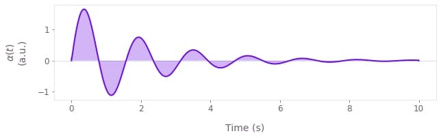
For example, to create an STF representing the function $\alpha(t) = 2 \sin(4 t) e^{-t/2}$, you can write

t = graph.identity_stf()
alpha = 2 * graph.sin(4 * t) * graph.exp(-t / 2)

which would look like this:

Manipulating STFs

As with PWCs, Boulder Opal graphs offer various STF-specific operations. You can also use mathematical operations with STFs (or operating STFs with Tensors) following the same rules outlined above for PWCs. You can learn more about these operations in the Understanding graphs in Boulder Opal topic.

Extracting STFs from a graph and plotting them

At variance with Tensors and PWCs, STFs do not have a name attribute, so you cannot directly export an STF from a graph. In order to export it, you need to either discretize it or sample it.

To discretize an STF, use the graph.discretize_stf operation, which will create a PWC approximation of it with the duration and number of samples you provide. You can export the PWC representing the discretized STF and plot it, for example, with qctrlvisualizer.plot_controls. You can see examples of this in this user guide or in our graphs tutorial.

Another option is to sample an STF using the graph.sample_stf operation and providing a list of sample times. This will provide you with a Tensor with the values of the STF at each sample time. Sampling it at N times will result in a tensor with shape batch_shape + (N,) + value_shape (see the attributes of STF nodes below). You can export this Tensor with the sampled STF values and plot it, for example, with qctrlvisualizer.plot_controls.

Attributes of STF nodes

STF nodes have two attributes that you can access in order to get information about them.

• value_shape: A tuple indicating the shape of the values of the function. This would be () for a signal, and, for example, (4,4) for an operator.

• batch_shape: A tuple indicating the shape of the batch in the function, allowing you to efficiently perform multiple parallel computations. You can learn more about batching in the Batching and broadcasting in Boulder Opal topic.

They do not have a values attribute because their values are not actually defined in a Tensor, unless they're sampled at some particular times. Similarly, STFs do not have a name attribute as they can't be directly fetched from a graph.

Converting between PWCs and STFs

As mentioned above, Boulder Opal graphs have operations to convert between the two time-dependent function types:

• graph.convolve_pwc creates a smooth STF by convolving a PWC with a kernel. With this operation you can generate smooth or band-limited pulses from a PWC function.

• graph.discretize_stf creates a PWC approximation of an STF, which you can export to easily visualize. The segment_count parameter of the operation indicates the number of segments of the resulting PWC. As such, a higher segment_count will result in a better approximation of the STF.

Next steps

For basic discussions of graphs, PWCs, and STFs, you can review our Understanding graphs in Boulder Opal topic or follow the Get familiar with graphs tutorial.

PWCs and STFs feature prominently in our user guides, which showcase a wide variety of applications where they can be used.

If you're looking for more advanced features, you can learn about broadcasting and batching, which are powerful tools to speed up calculations in Boulder Opal graphs.