Understand the library of signals

The controls used in quantum devices often take the form of signals that are variations over predefined shapes. For example, you can choose to embed your signal in a Gaussian envelope, to make sure that your controls evolve gradually from zero to their peak, and then back to zero again. Boulder Opal equips you predefined signal functions, to make it easier for you to create signals according to certain standardized shapes. With them, you only need to provide the minimum required number of parameters that characterize their shapes to create your signals.

In this topic, we discuss a library of signals suitable to be used with closed-loop optimization, because they can easily be exported to external quantum computing backends such as Qiskit, Pyquil, and QUA. We will explain how you can use this signal library and show examples of the signals that you can generate with it.

Note that Boulder Opal also has a library of signals incorporated in its graph framework and can therefore be used in optimization and simulation. You can learn more about it in this topic.

Signals library

Sometimes the kind of optimization that is right for you doesn't involve graphs, as explained in the Choosing a control design strategy in Boulder Opal topic. The library in boulderopal.signals contains functions that you can use for this kind of functionality, for instance, when dealing with closed-loop optimization. For example, suppose that you are interested in optimizing the width or amplitude of a Gaussian pulse used to achieve a certain gate in a real system. In this case, you can use signals from this library together with the Boulder Opal closed-loop optimization module to create different Gaussian-shaped signals and optimize them in your system.

You can access these signals through the boulderopal.signals module. The functions of this namespace return a Signal object, which contains the duration and shape of the signal. This Signal object can then be discretized and sampled to obtain a series of points that would be appropriate to export to a quantum computing backend with a particular sampling rate or time step.

For example, if you're sending your signals to a quantum computer that requires values sampled every 1 ns, you can use the method export_with_time_step(time_step=1e-9) to obtain an array of values of the signal that meets those requirements. You can then provide these values to the backend to apply this signal to the target quantum device. Similarly, if the quantum computing backend has a specific sampling rate, as opposed to a time step, you can obtain an array of numbers that is adequate to represent the signal for your backend by using the export_with_sampling_rate method of the Signal object.

As you have the liberty to also define the duration of the signal, it is possible that the time step that you provide during discretization might not exactly divide the duration of the signal that you passed. In this case, the total duration of the signal will be rounded up or down to the nearest value that corresponds to a multiple of the time steps. For the other parts of the discretization, the discretized samples correspond to the value of the signal at the middle of the segment that corresponds to the sample.

To learn more about the signals library, please read their reference documentation.

Signal types

The libraries of signals have similar kinds of signals shared among them. In the rest of this topic, we present an overview of the main types:

• Pulses: controls that go from zero to a peak, and then back to zero.
• Oscillations: controls that consist of oscillating functions that might have multiple peaks.
• Ramps: controls that monotonically vary from an initial value to a final value.

Pulses

These are signals that go (either asymptotically or strictly) from zero to a peak, and then back to zero. The Boulder Opal libraries of signals include these pulse types:

• Gaussian pulses (boulderopal.signals.gaussian_pulse).
• Hyperbolic secant pulses (boulderopal.signals.sech_pulse).
• Cosine pulses (boulderopal.signals.cosine_pulse).

The next figure illustrates what a hyperbolic secant pulse created with the Boulder Opal library of signals looks like.

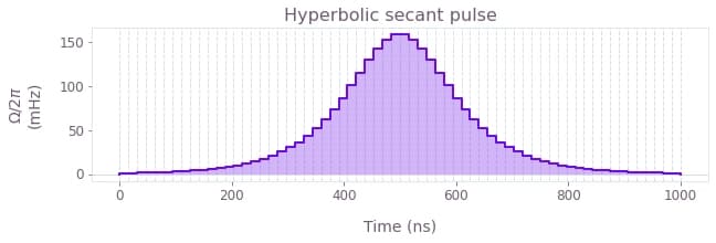
A particular case of these pulses is the square pulse, which has a finite value equal to its amplitude during a specified length of time, and is zero for all the rest of the time. To learn more about square pulses for Boulder Opal, see the reference documentation for boulderopal.signals.square_pulse.

Oscillations

It is possible to create pulses of many different shapes using superpositions of sines and cosines with different frequencies. In the Boulder Opal libraries of signals, these pulses can be found in the form of generic sinusoids or as a Hann series of squared sines with increasingly higher frequencies. To learn more about these oscillatory pulses, see the reference documentation for:

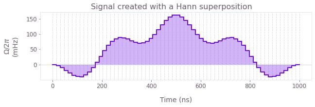
• Sinusoids (boulderopal.signals.sinusoid).
• Hann series (boulderopal.signals.hann_series).

The Hann series in particular can be used as a basis for pulses that are zero at the extremities. The following plot shows an example of a signal created with a Hann superposition.

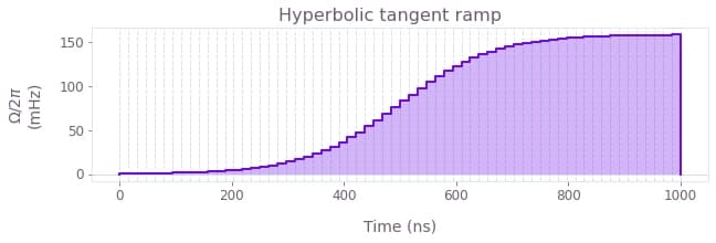
Ramps

Some signals of the signal library are continuously increasing or decreasing, instead of having a peak-like profile. These are called ramps, and you can learn more about them in the reference documentation for:

• Linear ramps (boulderopal.signals.linear_ramp).

• Hyperbolic tangent ramps (boulderopal.signals.tanh_ramp).

For further information about the signal library, take a look at its reference documentation.