plot_wigner_function
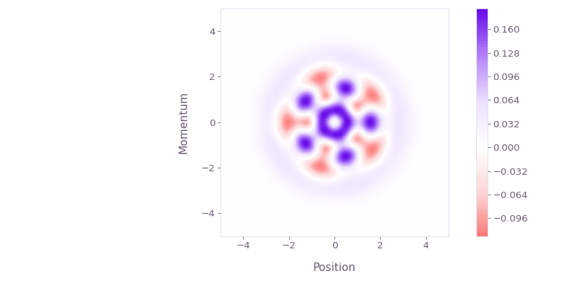
qctrlvisualizer.plot_wigner_function(wigner_function, position, momentum, contour_count=100, *, figure=None)Create a contour plot of the specified Wigner function.
Parameters
- wigner_function (np.ndarray) – The Wigner function values. Only the real part of this array will be plotted.
Must be a 2D array of shape
(L, K). - position (np.ndarray) – The dimensionless position vector. Must be a strictly increasing 1D array of length L.
- momentum (np.ndarray) – The dimensionless momentum vector. Must be a strictly increasing 1D array of length K.
- contour_count (int , optional) – The number of contour lines, the larger the value the finer the contour plot will be. Defaults to 100.
- figure (matplotlib.figure.Figure or None , optional) – A matplotlib Figure in which to place the plots. If passed, its dimensions and axes will be overridden.
Examples
Plot the Wigner function associated to state .
import numpy as np
import boulderopal as bo
from qctrlvisualizer import plot_wigner_function

position = np.linspace(-5, 5, 100)
momentum = np.linspace(-5, 5, 100)

graph = bo.Graph()

state = (graph.fock_state(10, 0) + graph.fock_state(10, 5)) / np.sqrt(2)
density_matrix = graph.outer_product(state, state)

wigner_transform = graph.wigner_transform(
    density_matrix, position, momentum, name="wigner_transform"
)

wigner_function = bo.execute_graph(
    graph=graph, output_node_names=["wigner_transform"]
)["output"]["wigner_transform"]["value"]

plot_wigner_function(wigner_function, position, momentum)