plot_filter_functions
qctrlvisualizer.plot_filter_functions(filter_functions, show_legend=True, x_axis_log=True, y_axis_log=True, *, figure=None)Create a plot of the specified filter functions.
Parameters
- filter_functions (dict) – The dictionary of filter functions to plot. The keys should be the names of the filter functions, and the values represent the filter functions by either a dictionary with the keys ‘frequencies’, ‘inverse_powers’, and optional ‘uncertainties’; or a list of samples as dictionaries with keys ‘frequency’, ‘inverse_power’, and optional ‘inverse_power_uncertainty’. The frequencies must be in Hertz an the inverse powers and their uncertainties in seconds. If the uncertainty of an inverse power is provided, it must be non-negative.
- show_legend (bool , optional) – Whether to add a legend to the plot. Defaults to True.
- x_axis_log (bool , optional) – Whether the x-axis is log-scale. Defaults to True.
- y_axis_log (bool , optional) – Whether the y-axis is log-scale. Defaults to True.
- figure (matplotlib.figure.Figure or None , optional) – A matplotlib Figure in which to place the plot. If passed, its dimensions and axes will be overridden.
Notes
For dictionary input, the key ‘inverse_power_uncertainties’ can be used instead of ‘uncertainties’. If both are provided then the value corresponding to ‘uncertainties’ is used. For list of samples input, the key ‘inverse_power_precision’ can be used instead of ‘inverse_power_uncertainty’. If both are provided then the value corresponding to ‘inverse_power_uncertainty’ is used.
As an example, the following is valid filter_functions input
filter_functions = {
    "Primitive": {
        "frequencies": [0.0, 1.0, 2.0],
        "inverse_powers": [15., 12., 3.],
        "uncertainties": [0., 0., 0.2],
    },
    "CORPSE": [
        {"frequency": 0.0, "inverse_power": 10.},
        {"frequency": 0.5, "inverse_power": 8.5},
        {"frequency": 1.0, "inverse_power": 5., "inverse_power_uncertainty": 0.1},
        {"frequency": 1.5, "inverse_power": 2.5},
    ],
}
Examples
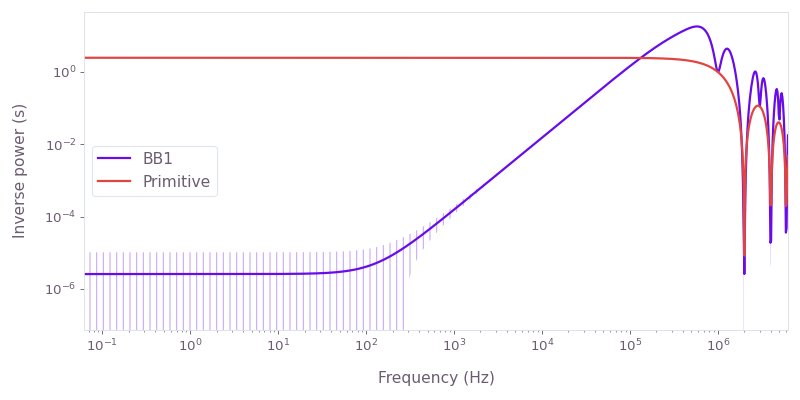
Compare the filter functions of a primitive control scheme to BB1. The primitive scheme is sensitive to amplitude noise, whereas BB1 suppresses amplitude noise. The Hamiltonian of the system is
where is the time-dependent Rabi rate implementing each control scheme and is a fractional time-dependent amplitude fluctuation process.
import numpy as np
import boulderopal as bo
from qctrlvisualizer import plot_filter_functions

graph = bo.Graph()

omega_max = 2 * np.pi * 1e6  # rad/s
frequencies = omega_max * np.logspace(-8, 0, 1000, base=10)
sample_count = 3000

primitive_duration = 5e-7  # s
primitive_hamiltonian = graph.hermitian_part(
    graph.constant_pwc(omega_max, primitive_duration) * graph.pauli_matrix("M")
)
graph.filter_function(
    control_hamiltonian=primitive_hamiltonian,
    noise_operator=primitive_hamiltonian,
    frequencies=frequencies,
    sample_count=sample_count,
    name="Primitive",
)

bb1_duration = 2.5e-6  # s
bb1_rates = omega_max * np.exp(1j * np.arccos(-1 / 4) * np.array([0, 1, 3, 3, 1]))
bb1_hamiltonian = graph.hermitian_part(
    graph.pwc_signal(bb1_rates, bb1_duration) * graph.pauli_matrix("M")
)
graph.filter_function(
    control_hamiltonian=bb1_hamiltonian,
    noise_operator=bb1_hamiltonian,
    frequencies=frequencies,
    sample_count=sample_count,
    name="BB1",
)

filter_function_result = bo.execute_graph(
    graph=graph, output_node_names=["Primitive", "BB1"], execution_mode="EAGER"
)["output"]

plot_filter_functions(filter_function_result)