How to run a Qiskit program using Fire Opal
An example of how to integrate Fire Opal with IBM hardware to run quantum phase estimation
You can use Fire Opal to quickly improve the results of circuits created using Qiskit. In this user guide we demonstrate how to add Fire Opal to your Qiskit experiment pipeline to improve the probablity of achieving successful results.
Example: Running quantum phase estimation with Fire Opal
1. Import libraries
The first step is to get your environment set up and download dependencies. To learn more read our How to set up your environment and install Fire Opal user guide.
import fireopal
import math
import qiskit
from qiskit_ibm_runtime import QiskitRuntimeService
from qctrlvisualizer import get_qctrl_style
import matplotlib.pyplot as plt
2. Set up quantum circuit
The creation of the circuit below is a minimal code version gathered from the Qiskit Quantum Phase Estimation tutorial.
The quantum phase estimation algorithm estimates the phase $\theta$ of the eigenvalue for a unitary operator $U$ applied to a quantum state $|\psi\rangle$, such that $U|\psi\rangle = \exp(2\pi i \theta)|\psi\rangle$. $n$ qubits are used to estimate $\theta$ to $n$ bits of precision. In this example, the state $|\psi\rangle = |1\rangle$, and the unitary operator rotates the state by an angle $\pi/4$, so $\theta = 1/8$.
def inverse_qft(qc, n):
    """Apply inverse quantum Fourier transform to the first n qubits in the circuit."""
    for qubit in range(n // 2):
        qc.swap(qubit, n - qubit - 1)
    for j in range(n):
        for m in range(j):
            qc.cp(-math.pi / float(2 ** (j - m)), m, j)
        qc.h(j)


qpe = qiskit.QuantumCircuit(4, 3)
qpe.x(3)
for qubit in range(3):
    qpe.h(qubit)

repetitions = 1
for counting_qubit in range(3):
    for i in range(repetitions):
        qpe.cp(math.pi / 4, counting_qubit, 3)
    repetitions *= 2

qpe.barrier()
inverse_qft(qpe, 3)  # Apply inverse QFT.
qpe.barrier()
for n in range(3):
    qpe.measure(n, n)

print(qpe)
┌───┐ ░ »
q_0: ┤ H ├─■──────────────────────────────────────────────────────────────░──X─»
├───┤ │ ░ │ »
q_1: ┤ H ├─┼────────■────────■────────────────────────────────────────────░──┼─»
├───┤ │ │ │ ░ │ »
q_2: ┤ H ├─┼────────┼────────┼────────■────────■────────■────────■────────░──X─»
├───┤ │P(π/4) │P(π/4) │P(π/4) │P(π/4) │P(π/4) │P(π/4) │P(π/4) ░ »
q_3: ┤ X ├─■────────■────────■────────■────────■────────■────────■────────░────»
└───┘ ░ »
c: 3/══════════════════════════════════════════════════════════════════════════»
»
« ┌───┐ ░ ┌─┐
«q_0: ┤ H ├─■──────────────■────────────────────────░─┤M├──────
« └───┘ │P(-π/2) ┌───┐ │ ░ └╥┘┌─┐
«q_1: ──────■────────┤ H ├─┼─────────■──────────────░──╫─┤M├───
« └───┘ │P(-π/4) │P(-π/2) ┌───┐ ░ ║ └╥┘┌─┐
«q_2: ─────────────────────■─────────■────────┤ H ├─░──╫──╫─┤M├
« └───┘ ░ ║ ║ └╥┘
«q_3: ──────────────────────────────────────────────░──╫──╫──╫─
« ░ ║ ║ ║
«c: 3/═════════════════════════════════════════════════╩══╩══╩═
« 0 1 2
3. Define function for plotting results
plt.style.use(get_qctrl_style())


def plot_histogram_of_probabilities(probabilites=None, counts=None, shot_count=None):
    """Plot a probability histogram from probability data or counts data"""
    probability_data = []
    if counts:
        assert (
            shot_count
        ), "Can not plot probability histogram with counts and without total shot count"
        bitstrings = sorted(counts.keys())
        probability_data = [counts[bitstring] / shot_count for bitstring in bitstrings]
    else:
        assert probabilites, "Can not plot without probability data"
        bitstrings = sorted(probabilites.keys())
        probability_data = [probabilites[bitstring] for bitstring in bitstrings]

    plt.figure(figsize=(15, 5))
    bars = plt.bar(bitstrings, probability_data)
    plt.xticks(rotation=90)
    plt.ylabel("Probability")
    plt.ylim([0, 1])
    plt.show()
4. Provide your device information and credentials
Next, we’ll provide device information for the real hardware backend. Fire Opal will execute the circuit on the backend on your behalf, and it is designed to work seamlessly across multiple backend providers.
For this example, we'll use an IBM Quantum API token. Visit IBM Quantum to sign up for an account and learn how to access systems with your account.
Use the obtained credentials to replace "your_IBMQ_token".
# These are the properties for the publicly available provider for IBM backends.
# If you have access to a private provider and wish to use it, replace these values.
hub = "ibm-q"
group = "open"
project = "main"
token = "YOUR_IBM_TOKEN"
credentials = fireopal.credentials.make_credentials_for_ibmq(
    token=token, hub=hub, group=group, project=project
)

service = QiskitRuntimeService(
    token=token, instance=hub + "/" + group + "/" + project, channel="ibm_quantum"
)
# Replace "desired_backend" with a device name
# Run fireopal.show_supported_devices() with your credentials to get a list of suppported backend names
backend_name = "desired_backend"5. Validate the circuit and backend
Now that we have defined our credentials and are able to select a device we wish to use, we can validate that Fire Opal can compile our circuit, and that it's compatible with the indicated backend.
Note that you may be prompted to authenticate your account with Fire Opal in a web browser.
validate_results = fireopal.validate(
    circuits=[qpe.qasm()], credentials=credentials, backend_name=backend_name
)


if validate_results["results"] == []:
    print("No errors found.")
else:
    print("The following errors were found:")
    for error in validate_results["results"]:
        print(error)
In this previous example, the output should be an empty list since there are no errors in the circuit, i.e. validate_results["results"] == []. Note that the length of the validate_results list is the total number of errors present across all circuits in a batch. Since our circuit is error free, we can execute our circuit on real hardware.
6 . Run experiment using Fire Opal
The execute function from Fire Opal accepts an OpenQASM representation of the quantum circuit, which is generated with the .qasm() method of Qiskit's QuantumCircuit class.
For more details, read the Fire Opal Get started guide.
shot_count = 2048

real_hardware_results = fireopal.execute(
    circuits=[qpe.qasm()],
    shot_count=shot_count,
    credentials=credentials,
    backend_name=backend_name,
)
bitstring_results = real_hardware_results["results"]
7. Show Fire Opal results
The execute function returns a list containing the results of each circuits that we ran. Since we only ran one circuit, its result is the first element of this list.
results = bitstring_results[0]

plot_histogram_of_probabilities(probabilites=results)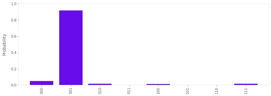
From the above plot, we observe that the bitstring with the highest probability is 001, which corresponds to
\begin{equation}\theta = \frac{(001)_2}{2^3} = \frac 18,\end{equation}
since our phase estimation circuit has $n = 3$ bits of precision. This is the result we expected. We can also compute the probability of getting the correct result.
print("Success probability = {:.2f}%".format(100.0 * results["001"]))Success probability = 91.65%
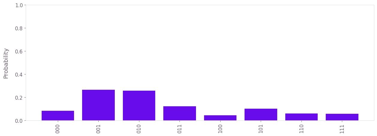
8. Compare results to running without Fire Opal
To get a true comparison, let's run the same circuit without Fire Opal. We'll run the circuit using Qiskit on the same IBM backend as used previously to get a one-to-one comparison.
backend = provider.get_backend(backend_name)

ibm_result = qiskit.execute(qpe, backend=backend, shots=shot_count).result()
ibm_counts = ibm_result.get_counts()
print(
"Success probability = {:.2f}%".format(
100.0 * ibm_counts["001"] / sum(ibm_counts.values())
)
)
plot_histogram_of_probabilities(counts=ibm_counts, shot_count=shot_count)Success probability = 26.56%
Congratulations! You've run a Qiskit program with Fire Opal and demonstrated the improvement it yielded on the quantum phase estimation algorithm.
Next up: Try out our tutorial on Creating and running circuits to run Fire Opal on Simon's Algorithm.
The package versions below were used to produce this notebook.
from fireopal import print_package_versions

print_package_versions()
| Package | Version |
| --------------------- | ------- |
| Python | 3.11.0 |
| networkx | 2.8.8 |
| numpy | 1.26.2 |
| sympy | 1.12 |
| fire-opal | 6.7.0 |
| qctrl-workflow-client | 2.2.0 |