How to run jobs on quantum hardware
Running jobs on quantum hardware using Fire Opal
Fire Opal provides a suite of functions for submitting jobs to quantum hardware or simulators, enabling efficient and optimized execution of quantum algorithms. This guide introduces and demonstrates five core functions for job submission: execute, iterate, estimate_expectation, iterate_expectation and solve_qaoa. Each function is tailored to the following use cases, allowing you to maximize the potential of your quantum resources:
executeis designed for a single circuit or a single list of circuitsestimate_expectationis a variant ofexecutethat estimates the expectation value of an executed circuit from a given set of observablesiterateis optimized for multi-job workloadsiterate_expectationis a variant ofiteratethat estimates the expectation value of an executed circuit from a given set of observables for multi-job workloadssolve_qaoaruns a hybrid quantum-classical workload and submits the hardware jobs required to reach an answer
1. Imports and initialization
To run these examples, you'll first need to set up your account information for Fire Opal, your hardware provider, and install the necessary packages into your environment using the following command.
pip install fire-opal qiskit pylatexenc numpy scipy networkx # Import necessary packages
import fireopal as fo
from fireopal.types import PauliOperator
from qiskit import QuantumCircuit, qasm3
from qiskit.circuit import Parameter
import numpy as np
import networkx as nx
from scipy.optimize import minimize# Replace "YOUR_QCTRL_API_KEY" with your API key, which you can find at https://accounts.q-ctrl.com/security
api_key = "YOUR_QCTRL_API_KEY"
fo.authenticate_qctrl_account(api_key=api_key)You can access devices on IBM Quantum via Fire Opal by signing up for an IBM Quantum account and using your token and credentials to authenticate.
# Insert your token and instance information
token = "YOUR_IBM_CLOUD_API_KEY"
instance = "YOUR_IBM_CRN"
# Create your credentials dictionary hardware platform authentication
credentials = fo.credentials.make_credentials_for_ibm_cloud(
    token=token, instance=instance
)
On Amazon Braket, you can use the function make_credentials_for_braket to generate the credentials dictionary needed to execute jobs.
arn = "your_role_arn"
credentials = fo.credentials.make_credentials_for_braket(arn=arn)
2. Running a single job in Fire Opal
2.1 Submitting a circuit with execute
The execute function is designed for direct execution of a single circuit or a single list of circuits. It applies Fire Opal’s error suppression pipeline to the circuits before submitting them to the specified quantum backend.
The following entanglement circuit demonstrates a basic example of how to code and run a job using the execute function. For a more in depth example of benchmarking a Bernstein–Vazirani with the execute function, see the Get started guide.
2.1.1 Create the circuit
# Create a basic circuit with a Hadamard and a CNOT gate
qc = QuantumCircuit(2)
qc.h(0)
qc.cx(0, 1)
qc.measure_all()
qc.draw("mpl")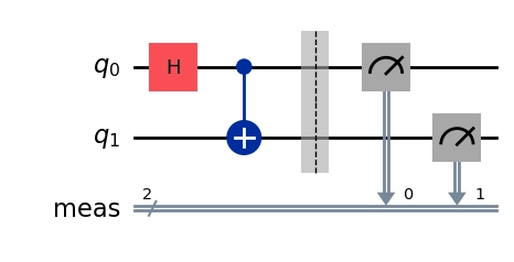
2.1.2 Submit the job
Be sure to choose a backend and replace "desired_backend" with the target name.
# Define shots and desired backend (replace "desired_backend" with your backend)
shot_count = 1024
backend_name = "desired_backend"
# Run the circuit with the execute function
fire_opal_job = fo.execute(
circuits=[qasm3.dumps(qc)],
shot_count=shot_count,
credentials=credentials,
backend_name=backend_name,
)2.1.3 Check status and retrieve result
# Check status
fire_opal_job.status()
The following function retrieves results or, if an error occurred, the corresponding error messages. The results contain the bitstring counts and the ID of the job submitted to the hardware provider.
You may also receive warnings if the device quality is degraded or experiencing significant fluctuations.
fire_opal_job.result(){'results': [{'00': 0.5058483621496975, '11': 0.4941516378503024}],
'provider_job_ids': ['d61qcrgkb74s739uv1og'],
'execution_results': [{'meas': {'00': 0.5058483621496975,
'11': 0.4941516378503024}}],
'execution_metadata': {'backend_name': 'ibm_brussels',
'circuit_metadata': [{'depth': 12,
'layout': [120, 121],
't1_times': {'120': 0.00025425820147614647, '121': 0.00030152189478855864},
't2_times': {'120': 0.00019065536901624432, '121': 0.00021874875131271818},
'gate_count': {'x': 1,
'rz': 9,
'sx': 5,
'ecr': 1,
'delay': 127,
'barrier': 1,
'measure': 2},
'shot_count': 1024,
'estimated_duration': 2.4000000000000003e-06,
'two_qubit_gate_error': {'(120,121)': {'ecr': 0.004730221248054056}},
'single_qubit_gate_error': {'120': {'x': 0.0001493738504645779,
'id': 0.0001493738504645779,
'rz': 0.0,
'sx': 0.0001493738504645779},
'121': {'x': 0.0002502735229580064,
'id': 0.0002502735229580064,
'rz': 0.0,
'sx': 0.0002502735229580064}}}],
'execution_timestamp': '2026-02-04T20:05:49.844584'}}
In the result payload, we can see the entry execution_metadata which contains information about the backend used to run the job and metadata about the circuit that was executed. This will provide a snapshot of the device characteristics at the time of execution.
fire_opal_job.result()["execution_metadata"]{'backend_name': 'ibm_brussels',
'circuit_metadata': [{'depth': 12,
'layout': [120, 121],
't1_times': {'120': 0.00025425820147614647, '121': 0.00030152189478855864},
't2_times': {'120': 0.00019065536901624432, '121': 0.00021874875131271818},
'gate_count': {'x': 1,
'rz': 9,
'sx': 5,
'ecr': 1,
'delay': 127,
'barrier': 1,
'measure': 2},
'shot_count': 1024,
'estimated_duration': 2.4000000000000003e-06,
'two_qubit_gate_error': {'(120,121)': {'ecr': 0.004730221248054056}},
'single_qubit_gate_error': {'120': {'x': 0.0001493738504645779,
'id': 0.0001493738504645779,
'rz': 0.0,
'sx': 0.0001493738504645779},
'121': {'x': 0.0002502735229580064,
'id': 0.0002502735229580064,
'rz': 0.0,
'sx': 0.0002502735229580064}}}],
'execution_timestamp': '2026-02-04T20:05:49.844584'}
Note that in the results shown above, one can see the legacy 'results' key which was standard prior to Fire Opal's support for multiple classical registers. The new key 'execution_results' has been added to support circuits with multiple classical measurements, where the return list will include one dictionary per classical register.
2.2 Submitting a circuit with estimate_expectation
The estimate_expectation function is designed to execute a single circuit or a single list of circuits and compute the expectation values of a given set of observables. Like execute, it also applies Fire Opal’s error suppression pipeline to the circuits before submitting them to the specified quantum backend.
The following code demonstrates a basic example of how to run a job using the estimate_expectation function. It prepares a circuit in a $|\Psi^+\rangle$ Bell state and estimates the expectation values of the $Z_0 \otimes Z_1$ and $X_0 \otimes X_1$ observables.
2.2.1 Create the circuit
# Create a basic circuit with a Hadamard and a CNOT gate
qc = QuantumCircuit(2)
qc.h(0)
qc.x(1)
qc.cx(0, 1)
qc.measure_all()
qc.draw("mpl")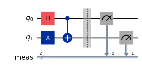
2.2.2 Create the observables
The estimate_expectation function requires a list of observables to estimate the expectation values of this circuit. You can build these observables using a list of Pauli strings.
observables = ["ZZ", "XX"]2.2.3 Submit the estimate_expectation job
Just like in execute, you choose a backend and replace "desired_backend" with the target name. Using a high shot_count will ensure the best accuracy of the expectation value estimation.
# Define shots and desired backend (replace "desired_backend" with your backend)
shot_count = 1024
backend_name = "desired_backend"
# Run the circuit with the estimate_expectation function
fire_opal_job = fo.estimate_expectation(
circuits=[qasm3.dumps(qc)],
shot_count=shot_count,
credentials=credentials,
backend_name=backend_name,
observables=observables,
)2.2.4 Check status and retrieve result
# Check status
fire_opal_job.status()
{'status_message': 'Job has been submitted to Q-CTRL.',
'action_status': 'STARTED'}
You will receive the expectation values and standard deviations corresponding to the list of observables defined above.
fire_opal_job.result(){'provider_job_id': 'cz19thjkvm9g008fp1j0',
'expectation_values': [-0.9921875, 0.990234375],
'standard_deviations': [0.12475562048961962, 0.13941263417767907]}
3. Running multiple jobs in Fire Opal
3.1 Submitting a circuit with iterate
The iterate function is optimized for use cases where you must submit multiple jobs, which generally fall into two categories: variational algorithms and batch workloads.
The following code demonstrates a basic example of using iterate to submit multiple jobs. You can also refer to more in depth guides on using iterate to run batch workloads and variational algorithms.
3.1.1 Create the circuit
Workloads that require multiple job submissions often leverage parameterized circuits, where the same circuit is executed with different parameter values. However, you can also use iterate to run non-parameterized circuits.
angle = Parameter("alpha")  # undefined number

# Create and optimize circuit once
param_qc = QuantumCircuit(1)
param_qc.rx(angle, 0)
param_qc.measure_all()
param_qc.draw("mpl")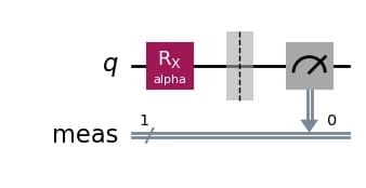
3.1.2 (Optional) Generate random parameters
# Generate sets of random values for the parameters
random_values = np.random.rand(500, 2)
parameter_dicts = [
    {param.name: val for param, val in zip(param_qc.parameters, values)}
    for values in random_values
]
3.1.3 Submit the job
# Define the backend (replace "desired_backend" with your backend)
backend_name = "desired_backend"

# Submit jobs for reach list of parameters
fire_opal_job = fo.iterate(
    circuits=[qasm3.dumps(param_qc)],
    shot_count=1024,
    credentials=credentials,
    backend_name=backend_name,
    parameters=parameter_dicts.tolist(),
)
3.1.4 Check status and retrieve results
Check the status of the job and retrieve results once the job has finished.
fire_opal_job.status()You can use the same result method to retrieve results or error messages.
results = fire_opal_job.result()Similar to the execute function, the results returned by iterate contain the bitstring counts and the ID of the job submitted to the hardware provider.
print(results["results"][0])
print(results["provider_job_ids"])
{'0': 0.9266282320022583, '1': 0.07337179780006409}
cytetqjy2gd000882y3g
3.2 Submitting a circuit with iterate_expectation
The iterate_expectation function is designed to execute multiple jobs and compute the expectation values of a given set of observables. Like in the previous functions, Fire Opal's error suppression pipeline is applied to all the circuits before submitting them to the specified quantum backend.
The following variational circuit demonstrates how to submit multiple jobs, obtaining a set of expectation values using iterate_expectation and using them to minimize a Hamiltonian.
3.2.1 Create the circuit
The variational state $|\psi(\theta, \phi)\rangle =\cos(\theta) \cos(\phi) |00\rangle + \cos(\theta) \sin(\phi) |01\rangle + \sin(\theta) \cos(\phi) |10\rangle + \sin(\theta) \sin(\phi) |11\rangle$ with parameters $\theta$ and $\phi$ is represented using the following circuit:
theta = Parameter("θ")
phi = Parameter("φ")
qc = QuantumCircuit(2)
qc.ry(2 * theta, 0)
qc.ry(2 * phi, 1)
qc.measure_all()
qc.draw("mpl")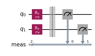
In this example the system Hamiltonian will be defined as $H = Z_0 \otimes I + I \otimes Z_1$ where $ Z_0 $ and $ Z_1 $ are the Pauli-Z operators acting on qubits 0 and 1, respectively.
3.2.2 Create the observables
The iterate_expectation function requires a list of observables to estimate the observation values of the circuit. Like estimate_expectation you can build these observables using a list of Pauli strings.
observables = PauliOperator.from_list([("ZI", 1), ("IZ", 1)])3.2.3 Submit the iterate_expectation job
When using the iterate_expectation function you can compute the observables $Z_0 \otimes I$ and $I \otimes Z_1$ directly from the variational circuit execution. Then you can add them to obtain the Hamiltonian and minimize it.
# Define the backend (replace "desired_backend" with your backend)
backend_name = "desired_backend"


def expectation_value(parameters):
    parameters_dict = {param.name: val for param, val in zip(qc.parameters, parameters)}
    job = fo.iterate_expectation(
        circuits=[qasm3.dumps(qc)],
        shot_count=1024,
        credentials=credentials,
        backend_name=backend_name,
        parameters=[parameters_dict],
        observables=observables,
    )
    return np.sum(job.result()["expectation_values"])
# Optimize θ and φ to minimize expectation value
result = minimize(
expectation_value,
x0=[np.pi / 4, np.pi / 4],
bounds=[(0, np.pi), (0, np.pi)],
method="COBYLA",
)
# Stop iterating after all circuits are sent
fo.stop_iterate(credentials, backend_name)
# Print results
print(f"Optimal θ: {result.x[0]:.4f}, Optimal φ: {result.x[1]:.4f}")
print(f"Minimum expectation value: {result.fun:.4f}")Optimal θ: 1.5978, Optimal φ: 1.5127
Minimum expectation value: -2.0000
4. Running hybrid quantum-classical optimization jobs with solve_qaoa
Fire Opal's solve_qaoa function invokes a fully-packaged QAOA solver, which automates all aspects of the Quantum Approximate Optimization Algorithm (QAOA) algorithm and optimizes each component for hardware execution.
Fire Opal repeatedly submits a quantum job and then uses a classical optimizer to optimize the set of inputs for the next quantum job. The algorithm continues this iteration process until convergence is reached.
The following example demonstrates the process of submitting a simple solve_qaoa job, which will run multiple quantum jobs with your chosen hardware provider. See how you can solve max-cut problems at full device scale using Fire Opal's QAOA solver, or define a custom cost function to solve any type of binary optimization problem.
4.1 Generate the optimization problem graph
The QAOA solver accepts either a graph or a polynomial cost function as problem definition. This example leverages a graph-based problem definition, which also requires defining the problem_type parameter.
# Define a random unweighted graph
graph = nx.random_regular_graph(d=3, n=36, seed=8)
nx.draw(graph, nx.kamada_kawai_layout(graph))
4.2 Submit the job
# Define the backend (replace "desired_backend" with your backend)
backend_name = "desired_backend"
# Run the QAOA solver
fire_opal_job = fo.solve_qaoa(
problem=graph,
credentials=credentials,
problem_type="maxcut",
backend_name=backend_name,
)This function performs multiple consecutive runs. Wait time may vary depending on hardware queues.
4.2 Check status and retrieve results
Since this function involves multiple quantum job executions, the results may be slightly delayed.
fire_opal_job.status(){'status_message': 'Job has been submitted to Q-CTRL.',
'action_status': 'STARTED'}
You can use the same function to retrieve results or error messages.
results = fire_opal_job.result()print(results["solution_bitstring"])
print(results["solution_bitstring_cost"])000010011011000110011100101111111000
-48.0
5. Advanced runtime options
The run_options parameter allows you to specify additional hardware provider-specific configurations. For example, you can input job tags that will be surfaced on the provider platform for easier tracking and management. You can also pass a session ID, to leverage an existing Qiskit Runtime Session, which enables you to maintain your position in the device queue across jobs executed both with and without Fire Opal.
Note: run_options are currently only supported for the IBM Quantum Platform.
run_options = fo.run_options.IbmRunOptions(
    job_tags=["your_job_tag"], session_id="your_session_id"
)

fire_opal_job = fo.execute(
    circuits=[qasm3.dumps(qc)],
    shot_count=shot_count,
    credentials=credentials,
    backend_name=backend_name,
    run_options=run_options,
)
from fireopal import print_package_versions
print_package_versions()| Package | Version |
| --------------------- | ------- |
| Python | 3.12.9 |
| networkx | 2.8.8 |
| numpy | 1.26.4 |
| sympy | 1.12.1 |
| fire-opal | 8.3.1 |
| qctrl-workflow-client | 5.3.1 |
