Compute the ground-state energy of formaldehyde using Fire Opal

Integrate Fire Opal into a quantum chemistry workflow for ground-state energy estimation

Computing the ground-state energy of a molecular system is a central task in electronic structure theory. From a classical perspective, high-accuracy methods such as Coupled Cluster with Singles and Doubles (CCSD) or multi-reference approaches can be used to obtain reliable reference energies, but their computational cost grows rapidly with system size and basis quality.

Quantum computing offers a complementary route, where you can map the molecular Hamiltonian to a qubit operator and use quantum circuits to approximate the ground state within the relevant fermionic Hilbert space. In this application note, you will solve the ground-state problem for formaldehyde ($\text{CH}_{2}\text{O}$), a small but chemically nontrivial molecule using Sample-based quantum diagonalization (SQD) eigenstate solver executed with and without Fire Opal. This application note covers the following:

An introduction to the $\text{CH}_{2}\text{O}$ electronic structure problem and active-space construction
An introduction to the SQD workflow
Execution of the eigenstate solver for $\text{CH}_{2}\text{O}$
Evaluation of the solver performance in terms of energy error

1. Introduction

You will compute the correlated ground-state energy of formaldehyde ($\text{CH}_{2}\text{O}$). The problem is formulated in a standard second-quantized setting, reduced to a chemically meaningful active space, and then mapped to a qubit Hamiltonian suitable for near-term processors. The Sample-based Quantum Diagonalization (SQD) solver uses bitstrings sampled from this Hamiltonian to reconstruct an approximate ground state. By executing the same SQD workflow with and without Fire Opal, you will obtain a controlled comparison of accuracy and robustness for a nontrivial, yet still classically tractable, molecular benchmark.

1.1 Electronic structure of formaldehyde ($\text{CH}_{2}\text{O}$)

Let's start with a standard quantum-chemistry pipeline. Given the formaldehyde's molecular geometry in the 3-21G basis set, a Hartree–Fock (HF) calculation provides a set of molecular orbitals, their occupations, and a mean-field ground-state energy. The Jordan–Wigner transformation is used to map the fermionic wavefunction of formaldehyde onto a qubit wavefunction that can be prepared on a quantum circuit. The JW mapping takes a system with $M$ spatial orbitals and represents it in a Hilbert space of $2M$ qubits, each spatial orbital is split into two spin orbitals, one for spin-up $\alpha$ and one for spin-down $\beta$, each represented by a single qubit.

For formaldehyde in the 3-21G basis, the Hartree–Fock calculation gives 22 spatial orbitals, $22\alpha+22\beta=44$ spin orbitals. Neutral $\text{CH}_{2}\text{O}$ has 16 electrons, and with a singlet reference $\text{spin}=0$ this corresponds to $8\alpha$ and $8\beta$ electrons. In the correlated calculation, the two lowest-energy spatial orbitals are frozen, they remain doubly occupied and do not participate in the calculation. This removes $4$ core electrons, leaving $12$ active electrons ($6\alpha$ and $6\beta$) distributed among the $20$ active spatial orbitals, or $40$ spin orbitals, so the quantum circuit effectively uses $40$ qubits to encode the electronic structure. The resulting fermionic Hilbert space has dimension $\binom{20}{6}^2 \approx 1.5 \times 10^9$, which is far too large for exact diagonalization.

1.2 Sample-based Quantum Diagonalization (SQD) workflow

To approximate the ground state of the $\text{CH}_{2}\text{O}$ Hamiltonian on a quantum device, the Sample-based Quantum Diagonalization (SQD) eigenstate solver is used, which combines a parameterized quantum circuit that explores relevant regions of Hilbert space with a classical subspace solver that reconstructs an approximate ground state from the sampled configurations. By working in a data-driven subspace determined directly from measurements on the device, SQD avoids the need to manipulate the full $2^N$-dimensional state vector while still capturing the dominant components of the ground state. The iterative nature of the method naturally provides diagnostics, such as orbital occupancy patterns, that can be used to assess whether the reconstructed state remains physically meaningful.

2. Imports and initializations

The following section sets up the necessary imports, credentials, and helper functions.

pip install qiskit_addon_sqd qctrlvisualizer pyscf

from qiskit import QuantumCircuit, qasm3
from qiskit_ibm_runtime import QiskitRuntimeService
from qiskit import QuantumCircuit, QuantumRegister
from qiskit.transpiler.preset_passmanagers import generate_preset_pass_manager
from qiskit_ibm_runtime import SamplerV2 as Sampler
from qiskit_addon_sqd.configuration_recovery import recover_configurations
from qiskit_addon_sqd.fermion import bitstring_matrix_to_ci_strs, solve_fermion
from qiskit_addon_sqd.subsampling import postselect_by_hamming_right_and_left, subsample
from qiskit_addon_sqd.counts import counts_to_arrays

import ffsim
from pyscf import cc
from pyscf.geomopt.geometric_solver import optimize
from pyscf import ao2mo, gto, mcscf, scf

import numpy as np
import fireopal as fo
import qctrlvisualizer as qv
import matplotlib.ticker as mticker
import matplotlib.pyplot as plt

2.1 Credentials and backend

This notebook is developed to run on an IBM backend. To run it, you need an IBM Quantum account. Set up Fire Opal with your IBM account information and choose a backend.

token = "YOUR_IBM_CLOUD_API_KEY"
instance = "YOUR_IBM_CRN"

credentials = fo.credentials.make_credentials_for_ibm_cloud(
    token=token, instance=instance
)

Q-CTRL authentication successful!

# Enter your desired IBM backend here.
service = QiskitRuntimeService()
backend = service.backend("your_desired_backend")

3. Molecular geometry and Hartree–Fock reference

You start by defining the formaldehyde molecule in a minimal but chemically meaningful setup. The Mole object specifies the nuclear geometry, the electronic structure model, and basic quantum numbers. The atomic positions correspond to a standard equilibrium geometry for $\text{CH}_{2}\text{O}$, with the oxygen and carbon placed along the $x$ axis and the two hydrogens arranged asymmetrically around the carbon, capturing the planar structure of the molecule. The total charge is set to zero and the spin multiplicity corresponds to a singlet state spin = 0, so the calculation describes neutral formaldehyde in its electronic ground state. A restricted Hartree–Fock (RHF) calculation is performed via scf.RHF(mol).run(). This provides the mean-field reference energy and the molecular orbital coefficients that are used in subsequent steps to construct the active-space Hamiltonian and its qubit representation.

# Formaldehyde
mol = gto.Mole()
mol.build(
    verbose=0,
    atom=[
        ["O", (0.6123, 0.0000, 0.0000)],
        ["C", (-0.6123, 0.0000, 0.0000)],
        ["H", (-1.2000, 0.2426, -0.8998)],
        ["H", (-1.2000, -0.2424, 0.8998)],
    ],
    basis="3-21G",
    spin=0,
    charge=0,
    symmetry=False,
)

mf = scf.RHF(mol).run()

<pyscf.gto.mole.Mole at 0x7cf6e9250e10>

The optimize routine takes the mean-field object mf as input and performs a geometry optimization using translation–rotation internal coordinates (TRIC). The resulting object contains the optimized nuclear positions used as the starting point for constructing the correlated Hamiltonian in the chosen active space.

mol_opt = optimize(mf, tol_grad=3e-4, verbose=0)  # Use geomeTRIC/TRIC under the hood

geometric-optimize called with the following command line:
/home/nemo/miniconda3/envs/q-chemistry/lib/python3.11/site-packages/ipykernel_launcher.py --f=/run/user/1000/jupyter/runtime/kernel-v3bb13e301defbc9bd1453787936876a3100b92123.json

                                        [91m())))))))))))))))/[0m                     
                                    [91m())))))))))))))))))))))))),[0m                
                                [91m*)))))))))))))))))))))))))))))))))[0m             
                        [94m#,[0m    [91m()))))))))/[0m                [91m.)))))))))),[0m          
                      [94m#%%%%,[0m  [91m())))))[0m                        [91m.))))))))*[0m        
                      [94m*%%%%%%,[0m  [91m))[0m              [93m..[0m              [91m,))))))).[0m      
                        [94m*%%%%%%,[0m         [93m***************/.[0m        [91m.)))))))[0m     
                [94m#%%/[0m      [94m(%%%%%%,[0m    [93m/*********************.[0m       [91m)))))))[0m    
              [94m.%%%%%%#[0m      [94m*%%%%%%,[0m  [93m*******/,[0m     [93m**********,[0m      [91m.))))))[0m   
                [94m.%%%%%%/[0m      [94m*%%%%%%,[0m  [93m**[0m              [93m********[0m      [91m.))))))[0m  
          [94m##[0m      [94m.%%%%%%/[0m      [94m(%%%%%%,[0m                  [93m,******[0m      [91m/)))))[0m  
        [94m%%%%%%[0m      [94m.%%%%%%#[0m      [94m*%%%%%%,[0m    [92m,/////.[0m       [93m******[0m      [91m))))))[0m 
      [94m#%[0m      [94m%%[0m      [94m.%%%%%%/[0m      [94m*%%%%%%,[0m  [92m////////,[0m      [93m*****/[0m     [91m,)))))[0m 
    [94m#%%[0m  [94m%%%[0m  [94m%%%#[0m      [94m.%%%%%%/[0m      [94m(%%%%%%,[0m  [92m///////.[0m     [93m/*****[0m      [91m))))).[0m
  [94m#%%%%.[0m      [94m%%%%%#[0m      [94m/%%%%%%*[0m      [94m#%%%%%%[0m   [92m/////)[0m     [93m******[0m      [91m))))),[0m
    [94m#%%%%##%[0m  [94m%%%#[0m      [94m.%%%%%%/[0m      [94m(%%%%%%,[0m  [92m///////.[0m     [93m/*****[0m      [91m))))).[0m
      [94m##[0m     [94m%%%[0m      [94m.%%%%%%/[0m      [94m*%%%%%%,[0m  [92m////////.[0m      [93m*****/[0m     [91m,)))))[0m 
        [94m#%%%%#[0m      [94m/%%%%%%/[0m      [94m(%%%%%%[0m      [92m/)/)//[0m       [93m******[0m      [91m))))))[0m 
          [94m##[0m      [94m.%%%%%%/[0m      [94m(%%%%%%,[0m                  [93m*******[0m      [91m))))))[0m  
                [94m.%%%%%%/[0m      [94m*%%%%%%,[0m  [93m**.[0m             [93m/*******[0m      [91m.))))))[0m  
              [94m*%%%%%%/[0m      [94m(%%%%%%[0m   [93m********/*..,*/*********[0m       [91m*))))))[0m   
                [94m#%%/[0m      [94m(%%%%%%,[0m    [93m*********************/[0m        [91m)))))))[0m    
                        [94m*%%%%%%,[0m         [93m,**************/[0m         [91m,))))))/[0m     
                      [94m(%%%%%%[0m   [91m()[0m                              [91m))))))))[0m       
                      [94m#%%%%,[0m  [91m())))))[0m                        [91m,)))))))),[0m        
                        [94m#,[0m    [91m())))))))))[0m                [91m,)))))))))).[0m          
                                 [91m()))))))))))))))))))))))))))))))/[0m             
                                    [91m())))))))))))))))))))))))).[0m                
                                         [91m())))))))))))))),[0m                     

-=# [1;94m geomeTRIC started. Version: 1.1 [0m #=-
Current date and time: 2025-11-27 22:44:01
#========================================================#
#| [92m    Arguments passed to driver run_optimizer():     [0m |#
#========================================================#
customengine              <pyscf.geomopt.geometric_solver.PySCFEngine object at 0x7cf65895f890> 
input                     /tmp/tmp2abw76ya/09ad8e40-f9ba-43da-99ef-02144fb147e9 
logIni                    /home/nemo/miniconda3/envs/q-chemistry/lib/python3.11/site-packages/pyscf/geomopt/log.ini 
maxiter                   100 
tol_grad                  0.0003 
verbose                   0 
----------------------------------------------------------
Custom engine selected.
Bonds will be generated from interatomic distances less than 1.20 times sum of covalent radii
12 internal coordinates being used (instead of 12 Cartesians)
Internal coordinate system (atoms numbered from 1):
Distance 1-2
Distance 2-3
Distance 2-4
Angle 1-2-4
Angle 3-2-4
Out-of-Plane 2-1-3-4
Translation-X 1-4
Translation-Y 1-4
Translation-Z 1-4
Rotation-A 1-4
Rotation-B 1-4
Rotation-C 1-4
<class 'geometric.internal.Distance'> : 3
<class 'geometric.internal.Angle'> : 2
<class 'geometric.internal.OutOfPlane'> : 1
<class 'geometric.internal.TranslationX'> : 1
<class 'geometric.internal.TranslationY'> : 1
<class 'geometric.internal.TranslationZ'> : 1
<class 'geometric.internal.RotationA'> : 1
<class 'geometric.internal.RotationB'> : 1
<class 'geometric.internal.RotationC'> : 1
> ===== Optimization Info: ====
> Job type: Energy minimization
> Maximum number of optimization cycles: 100
> Initial / maximum trust radius (Angstrom): 0.100 / 0.300
> Convergence Criteria:
> Will converge when all 5 criteria are reached:
>  |Delta-E| < 1.00e-06
>  RMS-Grad  < 3.00e-04
>  Max-Grad  < 4.50e-04
>  RMS-Disp  < 1.20e-03
>  Max-Disp  < 1.80e-03
> === End Optimization Info ===
Step    0 : Gradient = 2.059e-02/3.166e-02 (rms/max) Energy = -113.2208012969
Hessian Eigenvalues: 4.50000e-02 5.00000e-02 5.00000e-02 ... 3.34877e-01 3.34925e-01 9.33739e-01
Step    1 : Displace = [0m1.763e-02[0m/[0m2.236e-02[0m (rms/max) Trust = 1.000e-01 (=) Grad = [0m1.628e-03[0m/[0m1.923e-03[0m (rms/max) E (change) = -113.2218079630 ([0m-1.007e-03[0m) Quality = [0m0.942[0m
Hessian Eigenvalues: 4.50019e-02 5.00000e-02 5.00000e-02 ... 3.34867e-01 3.65172e-01 9.26718e-01
Step    2 : Displace = [0m4.070e-03[0m/[0m5.007e-03[0m (rms/max) Trust = 1.414e-01 ([92m+[0m) Grad = [0m1.187e-03[0m/[0m1.689e-03[0m (rms/max) E (change) = -113.2218095419 ([0m-1.579e-06[0m) Quality = [0m0.102[0m
Hessian Eigenvalues: 4.58079e-02 5.00000e-02 5.00000e-02 ... 3.32929e-01 5.47468e-01 9.12700e-01
Step    3 : Displace = [0m2.002e-03[0m/[0m2.530e-03[0m (rms/max) Trust = 2.035e-03 ([91m-[0m) Grad = [0m4.283e-04[0m/[0m5.995e-04[0m (rms/max) E (change) = -113.2218191912 ([0m-9.649e-06[0m) Quality = [0m0.865[0m
Hessian Eigenvalues: 4.56858e-02 5.00000e-02 5.00000e-02 ... 3.33057e-01 5.89147e-01 9.40664e-01
Step    4 : Displace = [92m1.133e-03[0m/[92m1.690e-03[0m (rms/max) Trust = 2.878e-03 ([92m+[0m) Grad = [0m3.888e-04[0m/[0m6.601e-04[0m (rms/max) E (change) = -113.2218190143 ([92m+1.769e-07[0m) Quality = [91m-0.148[0m
Hessian Eigenvalues: 4.99980e-02 5.00000e-02 5.00000e-02 ... 3.31688e-01 4.22814e-01 9.42406e-01
Step    5 : Displace = [92m5.493e-04[0m/[92m8.873e-04[0m (rms/max) Trust = 5.666e-04 ([91m-[0m) Grad = [92m1.596e-04[0m/[92m2.191e-04[0m (rms/max) E (change) = -113.2218199050 ([92m-8.907e-07[0m) Quality = [0m0.805[0m
Hessian Eigenvalues: 4.99980e-02 5.00000e-02 5.00000e-02 ... 3.31688e-01 4.22814e-01 9.42406e-01
Converged! =D

    #==========================================================================#
    #| If this code has benefited your research, please support us by citing: |#
    #|                                                                        |#
    #| Wang, L.-P.; Song, C.C. (2016) "Geometry optimization made simple with |#
    #| translation and rotation coordinates", J. Chem, Phys. 144, 214108.     |#
    #| http://dx.doi.org/10.1063/1.4952956                                    |#
    #==========================================================================#
    Time elapsed since start of run_optimizer: 15.797 seconds

With the optimized geometry you can recompute the restricted Hartree–Fock energy. To obtain a high-quality classical reference for the correlated ground-state energy, you can perform a CCSD calculation on the optimized Hartree–Fock reference, using a frozen-core approximation consistent with the active-space setup:

# Run the kernel to get the RHF energy
mf_opt = scf.RHF(mol_opt)
hf_e = float(mf_opt.kernel())
print(f"Restricted Hartree-Fock Energy: {hf_e}")

Restricted Hartree-Fock Energy: -113.22181990503708

ccsd = cc.CCSD(mf_opt).set(frozen=2).run()
exact_energy = ccsd.e_tot
print("CCSD reference energy:", exact_energy)

CCSD reference energy: -113.44730072803931

3.1 Active-space Hamiltonian and reference amplitudes

With the active-space definition, you can construct the corresponding many-body Hamiltonian and extract the integrals needed for the SQD solver.

open_shell = False
spin_sq = 0
n_frozen = 2
active_space = range(n_frozen, mol_opt.nao_nr())
num_orbitals = len(active_space)
n_electrons = int(sum(mf_opt.mo_occ[active_space]))
num_elec_a = (n_electrons + mol_opt.spin) // 2
num_elec_b = (n_electrons - mol_opt.spin) // 2
cas = mcscf.CASCI(mf_opt, num_orbitals, (num_elec_a, num_elec_b))
mo = cas.sort_mo(active_space, base=0)
hcore, nuclear_repulsion_energy = cas.get_h1cas(mo)
eri = ao2mo.restore(1, cas.get_h2cas(mo), num_orbitals)
t1 = ccsd.t1
t2 = ccsd.t2

To generate a trial state for the SQD workflow, you can use a unitary cluster Jastrow (UCJ) ansatz constructed from the CCSD single and double excitation amplitudes. The ffsim library provides a convenient interface for this through the UCJOpSpinBalanced operator, which builds a spin-balanced UCJ circuit tailored to the active-space Hamiltonian.

n_reps = 1
alpha_alpha_indices = [(p, p + 1) for p in range(num_orbitals - 1)]
alpha_beta_indices = [(p, p + 1) for p in range(num_orbitals - 1)]

ucj_op = ffsim.UCJOpSpinBalanced.from_t_amplitudes(
    t2=t2,
    t1=t1,
    n_reps=n_reps,
    interaction_pairs=(alpha_alpha_indices, alpha_beta_indices),
)
nelec = (num_elec_a, num_elec_b)

4. Circuit preparation

With the active-space Hamiltonian and the UCJ operator defined, you can now build the quantum circuit that prepares the trial state used for sampling in the SQD workflow. The circuit acts on a register of $2\,\text{num\_orbitals}$ qubits, corresponding to the $\alpha$ and $\beta$ spin orbitals in the active space, and is initialized in the Hartree–Fock configuration before the UCJ transformation is applied.

qubits = QuantumRegister(2 * num_orbitals, name="q")
circuit = QuantumCircuit(qubits)
circuit.append(ffsim.qiskit.PrepareHartreeFockJW(num_orbitals, nelec), qubits)
circuit.append(ffsim.qiskit.UCJOpSpinBalancedJW(ucj_op), qubits)
circuit.measure_all()

pass_manager = generate_preset_pass_manager(optimization_level=3, backend=backend)
isa_circuit = pass_manager.run(circuit)
print(f"Gate counts (w/o pre-init passes): {isa_circuit.count_ops()}")
pass_manager.pre_init = ffsim.qiskit.PRE_INIT
isa_circuit = pass_manager.run(circuit)
print(f"Gate counts (w/ pre-init passes): {isa_circuit.count_ops()}")

Pass: ContainsInstruction - 0.02122 (ms)Pass: UnitarySynthesis - 0.02456 (ms)Pass: HighLevelSynthesis - 101.91250 (ms)Pass: BasisTranslator - 0.17643 (ms)Pass: ElidePermutations - 0.01192 (ms)Pass: RemoveDiagonalGatesBeforeMeasure - 0.03171 (ms)Pass: RemoveIdentityEquivalent - 0.17881 (ms)Pass: InverseCancellation - 0.15092 (ms)Pass: ContractIdleWiresInControlFlow - 0.00715 (ms)Pass: CommutativeCancellation - 0.96846 (ms)Pass: ConsolidateBlocks - 8.52537 (ms)Pass: Split2QUnitaries - 0.01407 (ms)Pass: SetLayout - 0.00668 (ms)Pass: VF2Layout - 1.28508 (ms)Pass: BarrierBeforeFinalMeasurements - 0.51451 (ms)Pass: SabreLayout - 487.84590 (ms)Pass: CheckMap - 0.17428 (ms)Pass: VF2PostLayout - 1086.56836 (ms)Pass: ApplyLayout - 0.75722 (ms)Pass: FilterOpNodes - 0.62156 (ms)Pass: UnitarySynthesis - 0.01669 (ms)Pass: HighLevelSynthesis - 0.23365 (ms)Pass: BasisTranslator - 23.53239 (ms)Pass: Depth - 6.21009 (ms)Pass: Size - 0.01383 (ms)Pass: MinimumPoint - 0.01907 (ms)Pass: ConsolidateBlocks - 34.10459 (ms)Pass: UnitarySynthesis - 59.82471 (ms)Pass: RemoveIdentityEquivalent - 1.95932 (ms)Pass: Optimize1qGatesDecomposition - 14.50920 (ms)Pass: CommutativeCancellation - 16.81304 (ms)Pass: ContractIdleWiresInControlFlow - 0.01884 (ms)Pass: GatesInBasis - 2.93207 (ms)Pass: Depth - 3.53217 (ms)Pass: Size - 0.01526 (ms)Pass: MinimumPoint - 2.89083 (ms)Pass: ConsolidateBlocks - 41.71515 (ms)Pass: UnitarySynthesis - 23.73886 (ms)Pass: RemoveIdentityEquivalent - 0.95725 (ms)Pass: Optimize1qGatesDecomposition - 27.32229 (ms)Pass: CommutativeCancellation - 32.26256 (ms)Pass: ContractIdleWiresInControlFlow - 0.00978 (ms)Pass: GatesInBasis - 3.34454 (ms)Pass: Depth - 6.27613 (ms)Pass: Size - 0.01788 (ms)Pass: MinimumPoint - 13.30924 (ms)Pass: ConsolidateBlocks - 37.79292 (ms)Pass: UnitarySynthesis - 7.25460 (ms)Pass: RemoveIdentityEquivalent - 1.92499 (ms)Pass: Optimize1qGatesDecomposition - 9.87267 (ms)Pass: CommutativeCancellation - 15.27667 (ms)Pass: ContractIdleWiresInControlFlow - 0.01073 (ms)Pass: GatesInBasis - 2.11143 (ms)Pass: Depth - 2.46692 (ms)Pass: Size - 0.01550 (ms)Pass: MinimumPoint - 2.89059 (ms)Pass: ConsolidateBlocks - 22.40729 (ms)Pass: UnitarySynthesis - 7.41577 (ms)Pass: RemoveIdentityEquivalent - 0.94128 (ms)Pass: Optimize1qGatesDecomposition - 21.10672 (ms)Pass: CommutativeCancellation - 25.22111 (ms)Pass: ContractIdleWiresInControlFlow - 0.01431 (ms)Pass: GatesInBasis - 2.78139 (ms)Pass: Depth - 2.81262 (ms)Pass: Size - 0.01788 (ms)Pass: MinimumPoint - 0.01526 (ms)Pass: ConsolidateBlocks - 36.59749 (ms)Pass: UnitarySynthesis - 7.60293 (ms)Pass: RemoveIdentityEquivalent - 0.94342 (ms)Pass: Optimize1qGatesDecomposition - 7.11513 (ms)Pass: CommutativeCancellation - 29.15645 (ms)Pass: ContractIdleWiresInControlFlow - 0.01144 (ms)Pass: GatesInBasis - 2.70319 (ms)Pass: Depth - 9.57656 (ms)Pass: Size - 0.01335 (ms)Pass: MinimumPoint - 10.06651 (ms)Pass: ConsolidateBlocks - 50.69804 (ms)Pass: UnitarySynthesis - 17.57908 (ms)Pass: RemoveIdentityEquivalent - 1.05786 (ms)Pass: Optimize1qGatesDecomposition - 9.01985 (ms)Pass: CommutativeCancellation - 13.41367 (ms)Pass: ContractIdleWiresInControlFlow - 0.01240 (ms)Pass: GatesInBasis - 4.43721 (ms)Pass: Depth - 2.65527 (ms)Pass: Size - 0.01693 (ms)Pass: MinimumPoint - 0.01407 (ms)Pass: ConsolidateBlocks - 59.45563 (ms)Pass: UnitarySynthesis - 16.52598 (ms)Pass: RemoveIdentityEquivalent - 1.65534 (ms)Pass: Optimize1qGatesDecomposition - 22.98403 (ms)Pass: CommutativeCancellation - 33.03242 (ms)Pass: ContractIdleWiresInControlFlow - 0.01407 (ms)Pass: GatesInBasis - 1.99866 (ms)Pass: Depth - 7.59840 (ms)Pass: Size - 0.02432 (ms)Pass: MinimumPoint - 0.02217 (ms)Pass: ConsolidateBlocks - 34.21283 (ms)Pass: UnitarySynthesis - 18.53347 (ms)Pass: RemoveIdentityEquivalent - 0.92459 (ms)Pass: Optimize1qGatesDecomposition - 24.76335 (ms)Pass: CommutativeCancellation - 30.29871 (ms)Pass: ContractIdleWiresInControlFlow - 0.01121 (ms)Pass: GatesInBasis - 5.64694 (ms)Pass: Depth - 10.28943 (ms)Pass: Size - 0.01884 (ms)Pass: MinimumPoint - 0.01216 (ms)Pass: ConsolidateBlocks - 62.38580 (ms)Pass: UnitarySynthesis - 13.87620 (ms)Pass: RemoveIdentityEquivalent - 4.18258 (ms)Pass: Optimize1qGatesDecomposition - 29.88338 (ms)Pass: CommutativeCancellation - 9.11307 (ms)Pass: ContractIdleWiresInControlFlow - 0.00882 (ms)Pass: GatesInBasis - 2.06900 (ms)Pass: Depth - 3.16930 (ms)Pass: Size - 0.03076 (ms)Pass: MinimumPoint - 0.01645 (ms)Pass: VF2PostLayout - 781.11506 (ms)Pass: ContainsInstruction - 0.02766 (ms)Pass: InstructionDurationCheck - 0.01121 (ms)Pass: Decompose - 3.00145 (ms)Pass: MergeOrbitalRotations - 1.75023 (ms)Pass: UnitarySynthesis - 0.01740 (ms)Pass: HighLevelSynthesis - 41.18633 (ms)Pass: BasisTranslator - 0.16212 (ms)Pass: ElidePermutations - 0.01574 (ms)Pass: RemoveDiagonalGatesBeforeMeasure - 0.03266 (ms)Pass: RemoveIdentityEquivalent - 0.10657 (ms)Pass: InverseCancellation - 0.12231 (ms)Pass: ContractIdleWiresInControlFlow - 0.00644 (ms)Pass: CommutativeCancellation - 0.60129 (ms)Pass: ConsolidateBlocks - 2.79880 (ms)Pass: Split2QUnitaries - 0.01788 (ms)Pass: SetLayout - 0.01049 (ms)Pass: VF2Layout - 1.20568 (ms)Pass: BarrierBeforeFinalMeasurements - 0.42725 (ms)

Gate counts (w/o pre-init passes): OrderedDict([('sx', 8254), ('rz', 6923), ('cz', 3042), ('x', 500), ('measure', 40), ('barrier', 1)])


Pass: SabreLayout - 510.85472 (ms)Pass: CheckMap - 0.19765 (ms)Pass: VF2PostLayout - 175.64106 (ms)Pass: ApplyLayout - 0.82803 (ms)Pass: FilterOpNodes - 0.36907 (ms)Pass: UnitarySynthesis - 0.01335 (ms)Pass: HighLevelSynthesis - 0.15497 (ms)Pass: BasisTranslator - 8.40044 (ms)Pass: Depth - 2.19154 (ms)Pass: Size - 0.01073 (ms)Pass: MinimumPoint - 0.02050 (ms)Pass: ConsolidateBlocks - 15.45191 (ms)Pass: UnitarySynthesis - 26.01624 (ms)Pass: RemoveIdentityEquivalent - 0.71621 (ms)Pass: Optimize1qGatesDecomposition - 6.10590 (ms)Pass: CommutativeCancellation - 5.45287 (ms)Pass: ContractIdleWiresInControlFlow - 0.00978 (ms)Pass: GatesInBasis - 1.36399 (ms)Pass: Depth - 1.27196 (ms)Pass: Size - 0.00930 (ms)Pass: MinimumPoint - 1.31655 (ms)Pass: ConsolidateBlocks - 9.19533 (ms)Pass: UnitarySynthesis - 3.64876 (ms)Pass: RemoveIdentityEquivalent - 0.43750 (ms)Pass: Optimize1qGatesDecomposition - 3.54743 (ms)Pass: CommutativeCancellation - 5.38278 (ms)Pass: ContractIdleWiresInControlFlow - 0.00906 (ms)Pass: GatesInBasis - 1.37377 (ms)Pass: Depth - 1.03211 (ms)Pass: Size - 0.00739 (ms)Pass: MinimumPoint - 1.46317 (ms)Pass: ConsolidateBlocks - 8.11553 (ms)Pass: UnitarySynthesis - 3.71265 (ms)Pass: RemoveIdentityEquivalent - 0.45276 (ms)Pass: Optimize1qGatesDecomposition - 3.38793 (ms)Pass: CommutativeCancellation - 3.64780 (ms)Pass: ContractIdleWiresInControlFlow - 0.01025 (ms)Pass: GatesInBasis - 1.20711 (ms)Pass: Depth - 1.38736 (ms)Pass: Size - 0.01264 (ms)Pass: MinimumPoint - 2.06351 (ms)Pass: ConsolidateBlocks - 8.32605 (ms)Pass: UnitarySynthesis - 3.51977 (ms)Pass: RemoveIdentityEquivalent - 0.43988 (ms)Pass: Optimize1qGatesDecomposition - 3.06153 (ms)Pass: CommutativeCancellation - 3.60107 (ms)Pass: ContractIdleWiresInControlFlow - 0.00644 (ms)Pass: GatesInBasis - 1.19758 (ms)Pass: Depth - 0.95987 (ms)Pass: Size - 0.00930 (ms)Pass: MinimumPoint - 0.01168 (ms)Pass: VF2PostLayout - 1602.52237 (ms)Pass: ContainsInstruction - 0.02789 (ms)Pass: InstructionDurationCheck - 0.03958 (ms)

Gate counts (w/ pre-init passes): OrderedDict([('sx', 4555), ('rz', 3791), ('cz', 1646), ('x', 142), ('measure', 40), ('barrier', 1)])

sampler = Sampler(mode=backend)
job = sampler.run([isa_circuit], shots=10_000)

base_primitive._run:INFO:2025-11-27 22:47:29,267: Submitting job using options {'options': {}, 'version': 2, 'support_qiskit': True}

5. Running the algorithm

Run the $\text{CH}_{2}\text{O}$ UCJ trial circuit, with and without Fire Opal, to collect the measurement samples required for the SQD ground-state reconstruction.

# Run cell after IQX job completion
primitive_result = job.result()
pub_result = primitive_result[0]
counts_default = pub_result.data.meas.get_counts()

fire_opal_job = fo.execute(
    circuits=[qasm3.dumps(circuit.decompose(reps=5))],
    shot_count=10_000,
    credentials=credentials,
    backend_name=backend.name,
)

counts_fo = fire_opal_job.result()["results"][0]

6. SQD analysis and performance evaluation

The measurement data are now used as input to the SQD workflow. The function calculate_energies implements the full configuration-recovery and eigenstate-reconstruction loop: it converts the raw counts into bitstring and probability arrays, iteratively refines the configuration set using average orbital occupancies, and solves a sequence of reduced eigenvalue problems in the active-space sector.

rng = np.random.default_rng(24)
iterations = 3
samples_schedule = [600, 800, 1000, 1200, 1400]
experiments = len(samples_schedule)
n_batches = 5
max_davidson_cycles = 300

def calculate_energies(counts):
    bitstring_matrix_full, probs_arr_full = counts_to_arrays(counts)
    e_hist = np.zeros((experiments, iterations, n_batches))
    s_hist = np.zeros((experiments, iterations, n_batches))
    occupancy_hist = [[None for _ in range(iterations)] for _ in range(experiments)]

    for ex, spb in enumerate(samples_schedule):
        print(f"\n=== Experiment {ex} – samples_per_batch = {spb} ===")
        avg_occupancy = None
        for i in range(iterations):
            print(f"  Starting configuration recovery iteration {i}")
            if avg_occupancy is None:
                bs_mat_tmp = bitstring_matrix_full
                probs_arr_tmp = probs_arr_full
            else:
                bs_mat_tmp, probs_arr_tmp = recover_configurations(
                    bitstring_matrix_full,
                    probs_arr_full,
                    avg_occupancy,
                    num_elec_a,
                    num_elec_b,
                    rand_seed=rng,
                )
            postselected_bs_mat, postselected_probs_arr = (
                postselect_by_hamming_right_and_left(
                    bs_mat_tmp,
                    probs_arr_tmp,
                    hamming_right=num_elec_a,
                    hamming_left=num_elec_b,
                )
            )
            batches = subsample(
                postselected_bs_mat,
                postselected_probs_arr,
                samples_per_batch=spb,
                num_batches=n_batches,
                rand_seed=rng,
            )
            e_tmp = np.zeros(n_batches)
            s_tmp = np.zeros(n_batches)
            occs_tmp = []
            coeffs = []
            for j in range(n_batches):
                strs_a, strs_b = bitstring_matrix_to_ci_strs(batches[j])
                print(f"    Batch {j} subspace dimension: {len(strs_a) * len(strs_b)}")
                energy_sci, coeffs_sci, avg_occs, spin = solve_fermion(
                    batches[j],
                    hcore,
                    eri,
                    open_shell=open_shell,
                    spin_sq=spin_sq,
                    max_cycle=max_davidson_cycles,
                )
                energy_sci += nuclear_repulsion_energy
                e_tmp[j] = energy_sci
                print(f"    Energy {j}: {energy_sci}")
                s_tmp[j] = spin
                occs_tmp.append(avg_occs)
                coeffs.append(coeffs_sci)
            avg_occupancy = tuple(np.mean(occs_tmp, axis=0))
            e_hist[ex, i, :] = e_tmp
            s_hist[ex, i, :] = s_tmp
            occupancy_hist[ex][i] = avg_occupancy
    min_e = [np.min(e_hist[ex, -1, :]) for ex in range(experiments)]
    e_diff = [abs(e - exact_energy) for e in min_e]
    x1 = samples_schedule
    yt1 = [1.0, 1e-1, 1e-2, 1e-3, 1e-4, 1e-5]
    chem_accuracy = 0.001
    last_occ = occupancy_hist[-1][-1]
    y2 = last_occ[0] + last_occ[1]
    x2 = range(len(y2))
    return e_hist, min_e, e_diff, yt1, chem_accuracy, x1, y2, x2

# Convert counts into bitstring and probability arrays
e_hist_fo, min_e_fo, e_diff_fo, yt1_fo, chem_accuracy_fo, x1_fo, y2_fo, x2_fo = (
    calculate_energies(counts_fo)
)

=== Experiment 0 – samples_per_batch = 600 ===
  Starting configuration recovery iteration 0
    Batch 0 subspace dimension: 26896
    Energy 0: -113.2875885778956
    Batch 1 subspace dimension: 26896
    Energy 1: -113.2875885778956
    Batch 2 subspace dimension: 26896
    Energy 2: -113.2875885778956
    Batch 3 subspace dimension: 26896
    Energy 3: -113.2875885778956
    Batch 4 subspace dimension: 26896
    Energy 4: -113.2875885778956
  Starting configuration recovery iteration 1
    Batch 0 subspace dimension: 944784
    Energy 0: -113.38930801929412
    Batch 1 subspace dimension: 887364
    Energy 1: -113.38744860524812
    Batch 2 subspace dimension: 960400
    Energy 2: -113.35849912053587
    Batch 3 subspace dimension: 944784
    Energy 3: -113.39705880577881
    Batch 4 subspace dimension: 917764
    Energy 4: -113.39633464939948
  Starting configuration recovery iteration 2
    Batch 0 subspace dimension: 938961
    Energy 0: -113.37303988498914
    Batch 1 subspace dimension: 919681
    Energy 1: -113.39721546711228
    Batch 2 subspace dimension: 933156
    Energy 2: -113.37750594584291
    Batch 3 subspace dimension: 898704
    Energy 3: -113.40958540942141
    Batch 4 subspace dimension: 917764
    Energy 4: -113.39255176437467

=== Experiment 1 – samples_per_batch = 800 ===
  Starting configuration recovery iteration 0
    Batch 0 subspace dimension: 26896
    Energy 0: -113.2875885778956
    Batch 1 subspace dimension: 26896
    Energy 1: -113.2875885778956
    Batch 2 subspace dimension: 26896
    Energy 2: -113.2875885778956
    Batch 3 subspace dimension: 26896
    Energy 3: -113.2875885778956
    Batch 4 subspace dimension: 26896
    Energy 4: -113.2875885778956
  Starting configuration recovery iteration 1
    Batch 0 subspace dimension: 1597696
    Energy 0: -113.39304930080205
    Batch 1 subspace dimension: 1505529
    Energy 1: -113.42053694645612
    Batch 2 subspace dimension: 1547536
    Energy 2: -113.41426853784367
    Batch 3 subspace dimension: 1565001
    Energy 3: -113.40597830168264
    Batch 4 subspace dimension: 1580049
    Energy 4: -113.41215277160218
  Starting configuration recovery iteration 2
    Batch 0 subspace dimension: 1633284
    Energy 0: -113.41457064842888
    Batch 1 subspace dimension: 1560001
    Energy 1: -113.39599631150583
    Batch 2 subspace dimension: 1587600
    Energy 2: -113.41324919431219
    Batch 3 subspace dimension: 1525225
    Energy 3: -113.41421022080439
    Batch 4 subspace dimension: 1535121
    Energy 4: -113.40608012090325

=== Experiment 2 – samples_per_batch = 1000 ===
  Starting configuration recovery iteration 0
    Batch 0 subspace dimension: 26896
    Energy 0: -113.2875885778956
    Batch 1 subspace dimension: 26896
    Energy 1: -113.2875885778956
    Batch 2 subspace dimension: 26896
    Energy 2: -113.2875885778956
    Batch 3 subspace dimension: 26896
    Energy 3: -113.2875885778956
    Batch 4 subspace dimension: 26896
    Energy 4: -113.2875885778956
  Starting configuration recovery iteration 1
    Batch 0 subspace dimension: 2223081
    Energy 0: -113.41988799271988
    Batch 1 subspace dimension: 2268036
    Energy 1: -113.40607217363949
    Batch 2 subspace dimension: 2368521
    Energy 2: -113.40585572265165
    Batch 3 subspace dimension: 2280100
    Energy 3: -113.41236684677321
    Batch 4 subspace dimension: 2328676
    Energy 4: -113.42128937377414
  Starting configuration recovery iteration 2
    Batch 0 subspace dimension: 2353156
    Energy 0: -113.42244456256088
    Batch 1 subspace dimension: 2365444
    Energy 1: -113.41463436757597
    Batch 2 subspace dimension: 2347024
    Energy 2: -113.41897041893098
    Batch 3 subspace dimension: 2295225
    Energy 3: -113.40180814803554
    Batch 4 subspace dimension: 2304324
    Energy 4: -113.38958960167072

=== Experiment 3 – samples_per_batch = 1200 ===
  Starting configuration recovery iteration 0
    Batch 0 subspace dimension: 26896
    Energy 0: -113.2875885778956
    Batch 1 subspace dimension: 26896
    Energy 1: -113.2875885778956
    Batch 2 subspace dimension: 26896
    Energy 2: -113.2875885778956
    Batch 3 subspace dimension: 26896
    Energy 3: -113.2875885778956
    Batch 4 subspace dimension: 26896
    Energy 4: -113.2875885778956
  Starting configuration recovery iteration 1
    Batch 0 subspace dimension: 3193369
    Energy 0: -113.42801100400098
    Batch 1 subspace dimension: 3214849
    Energy 1: -113.4269231759451
    Batch 2 subspace dimension: 3236401
    Energy 2: -113.42484717301488
    Batch 3 subspace dimension: 3189796
    Energy 3: -113.42242835841776
    Batch 4 subspace dimension: 3243601
    Energy 4: -113.42542021227425
  Starting configuration recovery iteration 2
    Batch 0 subspace dimension: 3374569
    Energy 0: -113.42764822117307
    Batch 1 subspace dimension: 3211264
    Energy 1: -113.41503294551734
    Batch 2 subspace dimension: 3308761
    Energy 2: -113.42622169591407
    Batch 3 subspace dimension: 3139984
    Energy 3: -113.42485515013414
    Batch 4 subspace dimension: 3268864
    Energy 4: -113.42365017975288

=== Experiment 4 – samples_per_batch = 1400 ===
  Starting configuration recovery iteration 0
    Batch 0 subspace dimension: 26896
    Energy 0: -113.2875885778956
    Batch 1 subspace dimension: 26896
    Energy 1: -113.2875885778956
    Batch 2 subspace dimension: 26896
    Energy 2: -113.2875885778956
    Batch 3 subspace dimension: 26896
    Energy 3: -113.2875885778956
    Batch 4 subspace dimension: 26896
    Energy 4: -113.28758857789562
  Starting configuration recovery iteration 1
    Batch 0 subspace dimension: 4268356
    Energy 0: -113.4191921027971
    Batch 1 subspace dimension: 4116841
    Energy 1: -113.42314780175872
    Batch 2 subspace dimension: 4153444
    Energy 2: -113.42741127130701
    Batch 3 subspace dimension: 4048144
    Energy 3: -113.42628121795349
    Batch 4 subspace dimension: 4120900
    Energy 4: -113.42862408342738
  Starting configuration recovery iteration 2
    Batch 0 subspace dimension: 4145296
    Energy 0: -113.42754883432441
    Batch 1 subspace dimension: 4133089
    Energy 1: -113.4254154603791
    Batch 2 subspace dimension: 4289041
    Energy 2: -113.42883832619535
    Batch 3 subspace dimension: 4129024
    Energy 3: -113.42193330941731
    Batch 4 subspace dimension: 4243600
    Energy 4: -113.4281623463776

(
    e_hist_default,
    min_e_default,
    e_diff_default,
    yt1_default,
    chem_accuracy_default,
    x1_default,
    y2_default,
    x2_default,
) = calculate_energies(counts_default)

=== Experiment 0 – samples_per_batch = 600 ===
  Starting configuration recovery iteration 0
    Batch 0 subspace dimension: 9604
    Energy 0: -108.7451340647797
    Batch 1 subspace dimension: 9604
    Energy 1: -108.7451340647797
    Batch 2 subspace dimension: 9604
    Energy 2: -108.7451340647797
    Batch 3 subspace dimension: 9604
    Energy 3: -108.7451340647797
    Batch 4 subspace dimension: 9604
    Energy 4: -108.7451340647797
  Starting configuration recovery iteration 1
    Batch 0 subspace dimension: 1292769
    Energy 0: -111.94008269184971
    Batch 1 subspace dimension: 1283689
    Energy 1: -111.90964108773579
    Batch 2 subspace dimension: 1285956
    Energy 2: -111.61918103587362
    Batch 3 subspace dimension: 1301881
    Energy 3: -112.11324484954643
    Batch 4 subspace dimension: 1301881
    Energy 4: -111.60948309409991
  Starting configuration recovery iteration 2
    Batch 0 subspace dimension: 1140624
    Energy 0: -113.26509549780968
    Batch 1 subspace dimension: 1129969
    Energy 1: -113.25410141311288
    Batch 2 subspace dimension: 1121481
    Energy 2: -113.26183399427917
    Batch 3 subspace dimension: 1096209
    Energy 3: -113.31056596708696
    Batch 4 subspace dimension: 1098304
    Energy 4: -113.28203116572283

=== Experiment 1 – samples_per_batch = 800 ===
  Starting configuration recovery iteration 0
    Batch 0 subspace dimension: 9604
    Energy 0: -108.7451340647797
    Batch 1 subspace dimension: 9604
    Energy 1: -108.7451340647797
    Batch 2 subspace dimension: 9604
    Energy 2: -108.7451340647797
    Batch 3 subspace dimension: 9604
    Energy 3: -108.7451340647797
    Batch 4 subspace dimension: 9604
    Energy 4: -108.7451340647797
  Starting configuration recovery iteration 1
    Batch 0 subspace dimension: 2140369
    Energy 0: -112.51727168237161
    Batch 1 subspace dimension: 2244004
    Energy 1: -113.26518925387896
    Batch 2 subspace dimension: 2169729
    Energy 2: -112.04629322434131
    Batch 3 subspace dimension: 2178576
    Energy 3: -112.14023905686373
    Batch 4 subspace dimension: 2220100
    Energy 4: -111.87776259849824
  Starting configuration recovery iteration 2
    Batch 0 subspace dimension: 1982464
    Energy 0: -113.3191668568732
    Batch 1 subspace dimension: 2022084
    Energy 1: -113.34106783990188
    Batch 2 subspace dimension: 2036329
    Energy 2: -113.31949820511863
    Batch 3 subspace dimension: 1957201
    Energy 3: -113.3227064069527
    Batch 4 subspace dimension: 1979649
    Energy 4: -113.33444862042249

=== Experiment 2 – samples_per_batch = 1000 ===
  Starting configuration recovery iteration 0
    Batch 0 subspace dimension: 9604
    Energy 0: -108.7451340647797
    Batch 1 subspace dimension: 9604
    Energy 1: -108.7451340647797
    Batch 2 subspace dimension: 9604
    Energy 2: -108.7451340647797
    Batch 3 subspace dimension: 9604
    Energy 3: -108.7451340647797
    Batch 4 subspace dimension: 9604
    Energy 4: -108.7451340647797
  Starting configuration recovery iteration 1
    Batch 0 subspace dimension: 3411409
    Energy 0: -112.45510648564738
    Batch 1 subspace dimension: 3301489
    Energy 1: -111.89811835242475
    Batch 2 subspace dimension: 3258025
    Energy 2: -112.37038779001001
    Batch 3 subspace dimension: 3392964
    Energy 3: -111.86778609726969
    Batch 4 subspace dimension: 3359889
    Energy 4: -113.23606242669243
  Starting configuration recovery iteration 2
    Batch 0 subspace dimension: 2958400
    Energy 0: -113.37304053261217
    Batch 1 subspace dimension: 2924100
    Energy 1: -113.3381814894901
    Batch 2 subspace dimension: 2975625
    Energy 2: -113.36830669344843
    Batch 3 subspace dimension: 2944656
    Energy 3: -113.34623703652204
    Batch 4 subspace dimension: 2944656
    Energy 4: -113.34228018178595

=== Experiment 3 – samples_per_batch = 1200 ===
  Starting configuration recovery iteration 0
    Batch 0 subspace dimension: 9604
    Energy 0: -108.7451340647797
    Batch 1 subspace dimension: 9604
    Energy 1: -108.7451340647797
    Batch 2 subspace dimension: 9604
    Energy 2: -108.7451340647797
    Batch 3 subspace dimension: 9604
    Energy 3: -108.7451340647797
    Batch 4 subspace dimension: 9604
    Energy 4: -108.7451340647797
  Starting configuration recovery iteration 1
    Batch 0 subspace dimension: 4524129
    Energy 0: -112.36944341019313
    Batch 1 subspace dimension: 4713241
    Energy 1: -113.24469042038862
    Batch 2 subspace dimension: 4635409
    Energy 2: -113.28712874549532
    Batch 3 subspace dimension: 4631104
    Energy 3: -112.37552643490679
    Batch 4 subspace dimension: 4678569
    Energy 4: -112.30090822945243
  Starting configuration recovery iteration 2
    Batch 0 subspace dimension: 4157521
    Energy 0: -113.36276499352192
    Batch 1 subspace dimension: 4284900
    Energy 1: -113.3785175436852
    Batch 2 subspace dimension: 4251844
    Energy 2: -113.36505824729713
    Batch 3 subspace dimension: 4305625
    Energy 3: -113.36782435540138
    Batch 4 subspace dimension: 4260096
    Energy 4: -113.36533292786831

=== Experiment 4 – samples_per_batch = 1400 ===
  Starting configuration recovery iteration 0
    Batch 0 subspace dimension: 9604
    Energy 0: -108.7451340647797
    Batch 1 subspace dimension: 9604
    Energy 1: -108.7451340647797
    Batch 2 subspace dimension: 9604
    Energy 2: -108.7451340647797
    Batch 3 subspace dimension: 9604
    Energy 3: -108.7451340647797
    Batch 4 subspace dimension: 9604
    Energy 4: -108.7451340647797
  Starting configuration recovery iteration 1
    Batch 0 subspace dimension: 6330256
    Energy 0: -112.48005975566662
    Batch 1 subspace dimension: 6066369
    Energy 1: -112.32119785649384
    Batch 2 subspace dimension: 6255001
    Energy 2: -112.83436524458222
    Batch 3 subspace dimension: 6265009
    Energy 3: -112.54947014782984
    Batch 4 subspace dimension: 6155361
    Energy 4: -112.45773309441128
  Starting configuration recovery iteration 2
    Batch 0 subspace dimension: 5631129
    Energy 0: -113.3580204819709
    Batch 1 subspace dimension: 5560164
    Energy 1: -113.36852448354212
    Batch 2 subspace dimension: 5607424
    Energy 2: -113.36979135555231
    Batch 3 subspace dimension: 5645376
    Energy 3: -113.36601272012871
    Batch 4 subspace dimension: 5664400
    Energy 4: -113.37765089759762

To assess sample efficiency, you can compare the final SQD ground-state energy error as a function of the total number of measurement samples, with and without Fire Opal. For each point in the sampling schedule, the bar chart reports the absolute deviation from the CCSD reference energy (lower values indicate better performance) as a function of the maximum subspace dimension, following three rounds of classical configuration recovery. The subspace dimension indicates the classical computational resources allocated during the diagonalization step, larger dimensions require more classical computation but allow the solver to explore a richer basis of sampled configurations. Both execution methods are evaluated on the same backend with identical shot budgets to ensure a fair comparison.

The results reveal two principal trends. First, increasing the subspace dimension improves accuracy for both methods, since the classical solver gains access to a larger configuration space. Second, Fire Opal consistently achieves substantially lower error, approximately four times better across all tested subspace dimensions. This consistent improvement indicates that the use of Fire Opal enables the SQD solver to reconstruct a more accurate ground state from the same number of measurements.

plt.style.use(qv.get_qctrl_style())
samples = np.array(samples_schedule)
default_err = np.array(e_diff_default)
fo_err = np.array(e_diff_fo)
x = np.arange(len(samples))
width = 0.35
fig, ax = plt.subplots(figsize=(11, 8))

ax.bar(
    x + width / 2,
    fo_err,
    width,
    label="With Q-CTRL",
    alpha=0.8,
    edgecolor="black",
    linewidth=1.5,
)
ax.bar(
    x - width / 2,
    default_err,
    width,
    label="Without Q-CTRL",
    alpha=0.8,
    edgecolor="black",
    linewidth=1.5,
    color="gray",
)

max_subspace_dim = 2 * (samples**2)
max_subspace_dim_millions = max_subspace_dim / 1e6
x_labels = [f"{val:.1f}" for val in max_subspace_dim_millions]
ax.set_xticks(x)
ax.set_xticklabels(x_labels)
ax.set_xlabel("Maximum sub-space dimension [million]", fontsize=16)
ax.set_ylabel("Ground-state energy error [Ha]", fontsize=16)
ax.set_yticks([1e-2, 5e-2, 1e-1, 1.5e-1])
ax.yaxis.set_minor_locator(mticker.MultipleLocator(0.01))
ax.grid(True, which="major", axis="y", linestyle="--", linewidth=0.8, alpha=0.7)
ax.grid(True, which="minor", axis="y", linestyle=":", linewidth=0.8, alpha=0.4)
ax.set_title(r"Formaldehyde (CH$_2$O) – Energy Error vs Samples", fontsize=20)
ax.legend(
    title="Execution",
    labels=["With Q-CTRL", "Without Q-CTRL"],
    fontsize=16,
    title_fontsize=16,
)
ax.annotate(
    "",
    xy=(0.62, 0.88),
    xytext=(0.20, 0.88),
    xycoords="axes fraction",
    textcoords="axes fraction",
    arrowprops=dict(arrowstyle="-|>", mutation_scale=24, linewidth=4),
)
ax.text(
    0.4,
    0.9,
    "Increasing classical resources",
    transform=ax.transAxes,
    ha="center",
    va="bottom",
    fontsize=16,
)
ax.annotate(
    "",
    xy=(-0.14, 0.32),
    xytext=(-0.14, 0.65),
    xycoords="axes fraction",
    textcoords="axes fraction",
    arrowprops=dict(arrowstyle="->", mutation_scale=22, linewidth=4),
)
ax.text(
    -0.16,
    0.5,
    "Lower is better",
    transform=ax.transAxes,
    ha="center",
    va="center",
    rotation=90,
    fontsize=16,
)
with np.errstate(divide="ignore", invalid="ignore"):
    factors = np.where(fo_err > 0, default_err / fo_err, np.nan)
best_idx = np.nanargmax(factors)
best_factor = factors[best_idx]
x_best = x[best_idx] + width / 2
y_best = fo_err[best_idx]
y_default = default_err[best_idx]
ax.annotate(
    f"{best_factor:.1f}X",
    xy=(x_best, y_best),
    xytext=(x_best, y_default),
    ha="center",
    va="bottom",
    fontsize=20,
    arrowprops=dict(arrowstyle="->", mutation_scale=22, linewidth=4),
)
plt.tight_layout()
plt.show()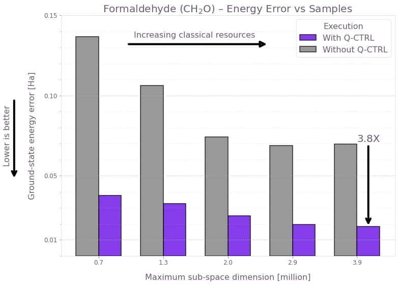

The following package versions were used to produce this notebook.

fo.print_package_versions()

| Package               | Version |
| --------------------- | ------- |
| Python                | 3.11.14 |
| matplotlib            | 3.10.8  |
| networkx              | 3.5     |
| numpy                 | 2.3.4   |
| qiskit                | 2.2.3   |
| qiskit-ibm-runtime    | 0.43.1  |
| sympy                 | 1.14.0  |
| fire-opal             | 9.1.0   |
| qctrl-visualizer      | 9.0.0   |
| qctrl-workflow-client | 7.3.0   |