Solve the Transverse-Field Ising Model using Fire Opal
Using Fire Opal's estimate_expectation to solve TFIM
The Transverse-field Ising Model (TFIM) is widely used to study quantum spin systems and phase transitions. It describes a lattice of quantum spins with nearest-neighbor interactions and an external magnetic field applied perpendicular to the spin alignment axis. Simulating the Transverse-field Ising Model is a challenging task due to noise and decoherence. Fire Opal's estimate_expectation function provides an optimized calculation of single-qubit magnetizations, enhancing the solution of the TFIM on real hardware devices.
This application note provides a practical example of TFIM implementation, covering the following:
- Implementing the TFIM Hamiltonian on a graph of connected spin triangles
- Simulating time evolution using Trotterized circuits under varying depths
- Estimating and visualizing single-qubit magnetizations $\langle 𝑍_𝑖 \rangle$ over time
- Comparing results with and without Fire Opal’s error suppression
Ultimately, this example highlights Fire Opal’s ability to improve signal fidelity in quantum many-body simulations.
1. Introduction
The Transverse-field Ising Model (TFIM) is a quantum spin model that captures essential features of quantum phase transitions. The Hamiltonian is defined as:
\begin{equation} H = -J \sum_{i} Z_i Z_{i+1} - h \sum_{i} X_i \end{equation}
where $Z_i$ and $X_i$ are Pauli operators acting on qubit $i$, $J$ is the coupling strength between neighboring spins, and $h$ is the strength of the transverse magnetic field. The first term represents classical ferromagnetic interactions, while the second introduces quantum fluctuations through the transverse field. To simulate TFIM dynamics, you use a Trotter decomposition of the unitary evolution operator $e^{-iHt}$, implemented through layers of RX and RZZ gates based on a custom graph of connected spin triangles. The simulation explores how magnetization $\langle Z \rangle$ evolves with increasing Trotter steps.
TFIM implementation performance is obtained by comparing noiseless simulations with noisy backends. Fire Opal’s enhanced execution and error suppression features are used to mitigate the effect of noise in real hardware, yielding more reliable estimates of spin observables like $\langle Z_i \rangle$ and correlators $\langle Z_i Z_j \rangle$.
2. Imports and initialization
You can find detailed guidelines for setting up your development environment. You can install the necessary packages using the following pip command.
pip install fire-opal qiskit pylatexenc qiskit-aer networkximport numpy as np
import networkx as nx
import fireopal as fo
from qiskit import QuantumCircuit
from qiskit import qasm3
import matplotlib.pyplot as plt
from qiskit_aer import AerSimulatorTo use Fire Opal within your local development environment you should authenticate using an API key.
api_key = "YOUR_QCTRL_API_KEY"
fo.authenticate_qctrl_account(api_key=api_key)

# Set credentials.
token = "YOUR_IBM_CLOUD_API_KEY"
instance = "YOUR_IBM_CRN"

credentials = fo.credentials.make_credentials_for_ibm_cloud(
    token=token, instance=instance
)
Q-CTRL authentication successful!
3. Set up the problem
3.1. Generate the TFIM Graph
First you need to create the lattice of quantum spins, defining the spin-spin coupling. In this particular case, you will generate an adjacency matrix for a graph composed of $n$ connected triangles arranged as a linear chain. Each triangle is formed by three fully connected nodes, creating a closed loop. The function connected_triangles_adj_matix generates this graph, linking the first node of each new triangle with the last node of the previous one leading to a total of $2n+1$ nodes.
def connected_triangles_adj_matrix(n):
    """
    Generate the adjacency matrix for 'n' connected triangles in a chain.
    """
    num_nodes = 2 * n + 1
    adj_matrix = np.zeros((num_nodes, num_nodes), dtype=int)

    for i in range(n):
        a, b, c = i * 2, i * 2 + 1, i * 2 + 2  # Nodes of the current triangle

        # Connect the three nodes in a triangle
        adj_matrix[a, b] = adj_matrix[b, a] = 1
        adj_matrix[b, c] = adj_matrix[c, b] = 1
        adj_matrix[a, c] = adj_matrix[c, a] = 1

        # If not the first triangle, connect to the previous triangle
        if i > 0:
            adj_matrix[a, a - 1] = adj_matrix[a - 1, a] = 1

    return adj_matrix
3.2 Color Graph Edges
Given a graph representing the spin interaction lattice, the function edge_coloring provides a way to identify sets of non-overlapping edges. It converts the graph to a line graph, where each node corresponds to an edge in the original graph. It then performs a coloring of the line graph so that adjacent edges are assigned different colors.
def edge_coloring(graph):
    """
    Takes a NetworkX graph and returns a list of lists where each inner list contains
    the edges assigned the same color.
    """
    line_graph = nx.line_graph(graph)
    edge_colors = nx.coloring.greedy_color(line_graph)

    color_groups = {}
    for edge, color in edge_colors.items():
        if color not in color_groups:
            color_groups[color] = []
        color_groups[color].append(edge)

    return list(color_groups.values())
3.3 Generate Trotterized Circuits on Spin Graphs
To simulate quantum dynamics governed by the Transverse-field Ising Model (TFIM), the function generate_tfim_circ_custom_graph constructs a Trotterized quantum circuit from an arbitrary spin interaction graph. It implements the time evolution operator:
\begin{equation} e^{-i H t}, \quad \text{with} \quad H = -J \sum_{\langle i,j \rangle} Z_i Z_j - h \sum_i X_i, \end{equation}
using second-order Trotter decomposition. The evolution is split into alternating layers of local rotations using RX gates for the transverse field and entangling interactions using RZZ gates for spin-spin couplings. The gate angles are determined by the simulation time step dt, the transverse field strength h, and the coupling constant J. The produced circuit simulates TFIM dynamics across various depths and configurations and is used repeatedly across different Trotter step counts to analyze magnetization evolution.
def generate_tfim_circ_custom_graph(
    steps, h, J, dt, psi0, graph: nx.graph.Graph, meas_basis="Z", mirror=False
):
    """
    Generate a second order trotter of the form e^(a+b) ~ e^(b/2) e^a e^(b/2) for simulating a transverse field ising model:
    e^{-i H t} where the Hamiltonian H = -J \\sum_i Z_i Z_{i+1} + h \\sum_i X_i.

    steps: Number of trotter steps
    theta_x: Angle for layer of X rotations
    theta_zz: Angle for layer of ZZ rotations
    theta_x: Angle for second layer of X rotations
    J: Coupling between nearest neighbouring spins
    h: The transverse magnetic field strength
    dt: t/total_steps
    psi0: initial state (assumed to be prepared in the computational basis).
    meas_basis: basis to meaasure all correlators in

    This is a second order trotter of the form e^(a+b) ~ e^(b/2) e^a e^(b/2)
    """
    theta_x = h * dt
    theta_zz = -2 * J * dt
    qubit_count = graph.number_of_nodes()
    color_edges = edge_coloring(graph)
    circ = QuantumCircuit(qubit_count, qubit_count)
    # Initial state, for typical cases in the computational basis
    for i, b in enumerate(psi0):
        if b == "1":
            circ.x(i)
    # Trotter steps
    for step in range(steps):
        for i in range(qubit_count):
            circ.rx(theta_x, i)
        if mirror:
            color_edges = [sublist[::-1] for sublist in color_edges[::-1]]
        for edge_list in color_edges:
            for edge in edge_list:
                circ.rzz(theta_zz, edge[0], edge[1])
        for i in range(qubit_count):
            circ.rx(theta_x, i)

    # some typically used basis rotations
    if meas_basis == "X":
        for b in range(qubit_count):
            circ.h(b)
    elif meas_basis == "Y":
        for b in range(qubit_count):
            circ.sdg(b)
            circ.h(b)

    for i in range(qubit_count):
        circ.measure(i, i)

    return circ


def trotter_circuits(G, d_ind_tot, J, h, dt, meas_basis, mirror=True):
    """
    Generates a sequence of Trotterized circuits, each with increasing depth.
    Given a spin interaction graph and Hamiltonian parameters, it constructs
    a list of circuits with 1 to d_ind_tot Trotter steps

    G: Graph defining spin interactions (edges = ZZ couplings)
    d_ind_tot: Number of Trotter steps (maximum depth)
    J: Coupling between nearest neighboring spins
    h: Transverse magnetic field strength
    dt: (t / total_steps
    meas_basis: Basis to measure all correlators in
    mirror: If True, mirror the Trotter layers
    """
    qubit_count = len(G)
    circuits = []
    psi0 = "0" * qubit_count

    for steps in range(1, d_ind_tot + 1):
        circuits.append(
            generate_tfim_circ_custom_graph(
                steps, h, J, dt, psi0, G, meas_basis, mirror
            )
        )
    return circuits
3.2 Estimate Single-Qubit Magnetizations ⟨Zᵢ⟩
To analyze the magnetization dynamics of the Transverse-field Ising Model, you need to compute the expectation value of the Pauli-Z operator on each individual qubit. For the exact simulation you will use the function z_expectation to compute the magnetization $\langle Z_i \rangle$ from bitstring measurement results. For real devices, Fire Opal's estimate_expectation function evaluates the magnetization expectation values from a dictionary defining the specific qubit $i$. These methods are necessary for assessing local magnetization and tracking the time evolution of spin observables in quantum circuits.
def z_expectation(counts: dict[str, int], index: int):
    """
    counts: Dict of mitigated bitstrings.
    index: Index i in the single operator expectation value < II...Z_i...I > to be calculated.
    return:  < Z_i >
    """
    z_exp = 0
    tot = 0
    for bitstring, value in counts.items():
        sum = int(bitstring[index])
        sign = 1
        if sum % 2 == 1:
            sign = -1
        z_exp += sign * value
        tot += value

    return z_exp / tot
def generate_z_observables(qubit_count: int):
observables = []
for i in range(qubit_count):
pauli_string = "".join(["Z" if j == i else "I" for j in range(qubit_count)])
observables.append((pauli_string, 1))
return observables4. Run the algorithm
4.1 Selecting the quantum device
Choose a backend from the supported devices your IBM account has access to, and replace desired_backend with the target name. In this application note you will use the statevector simulator to as baseline, this will not be suitable for circuits with large number of qubits.
backend_name = "desired_backend"
backend_sim = AerSimulator(method="statevector")
4.2 Build and running the Trotterized circuits
You need to define the parameters for generating the Trotterized circuits that simulate the Transverse-field Ising Model (TFIM) on the graph of connected spin triangles. In this case, the lattice is composed of a chain of 12 triangles arranged linearly producing a 25-qubit system.
circs = []
for num_triangles in [12]:
    for meas_basis in ["Z"]:
        A = connected_triangles_adj_matrix(num_triangles)
        G = nx.from_numpy_array(A)
        qubit_count = len(G)
        d_ind_tot = 21
        dt = 2 * np.pi * 1 / 30 * 0.5
        J = 1
        h = -4
        circs.extend(trotter_circuits(G, d_ind_tot, J, h, dt, meas_basis, True))
4.3 Calculate Magnetization Dynamics
4.3.1 Exact Simulations
To calculate observables from exact simulations, the circuit list circ_list is executed on the statevector simulator using run_sim, which runs each circuit with $4096$ shots and normalizes the raw bitstring counts via normalize_counts. These normalized results are then passed to make_cors, which computes single-qubit Z expectation values ⟨Zᵢ⟩ at each Trotter step (d_ind_tot), then averages these Z values over all qubits, returning a 1D array sim that summarizes the magnetization dynamics over time.
def normalize_counts(counts_list, shots):
    new_counts_list = []
    for counts in counts_list:
        a = {k: v / shots for k, v in counts.items()}
        new_counts_list.append(a)
    return new_counts_list
def run_sim(circ_list):
shots = 4096
res = backend_sim.run(circ_list, shots=shots)
normed = normalize_counts(res.result().get_counts(), shots)
return normedsim_counts = run_sim(circs)def make_cors(counts, qubit_count):
d_ind_tot = 21
mz = np.empty((qubit_count, d_ind_tot)) # <Z_i>
for d_ind in range(d_ind_tot):
counts = counts[d_ind]
for i in range(qubit_count):
mz[i, d_ind] = z_expectation(counts, i)
average_z = np.mean(mz, axis=0)
return np.concatenate((np.array([1]), average_z), axis=0)sim = make_cors(sim_counts[0:21], qubit_count=21)4.3.2 Real Devices
To evaluate magnetization dynamics on real quantum hardware, the circuits are executed on the selected IBM backend using Fire Opal’s estimate_expectation function. The Trotter-evolved circuits are divided into two batches to be run on the QPU. Each batch is submitted with $4096$ shots, and Pauli-Z observables are measured across all qubits using the dictionary generated by generate_z_observables. The resulting expectation values are concatenated and grouped by Trotter step. The average over qubits for each step is calculated, obtaining the observed magnetization evolution from real-device execution.
fire_opal_job_A = fo.estimate_expectation(
    circuits=[qasm3.dumps(qc) for qc in circs[:11]],
    shot_count=4096,
    credentials=credentials,
    backend_name=backend_name,
    observables=generate_z_observables(qubit_count),
)
fire_opal_job_B = fo.estimate_expectation(
    circuits=[qasm3.dumps(qc) for qc in circs[11:]],
    shot_count=4096,
    credentials=credentials,
    backend_name=backend_name,
    observables=generate_z_observables(qubit_count),
)
Now group the resulting expectation values by Trotter step and concatenate to make averaging easier. The average values obtained give us the observed magnetization evolution from real-device execution.
jobs = (
    fire_opal_job_A.result()["expectation_values"]
    + fire_opal_job_B.result()["expectation_values"]
)
jobs_Hlist = [jobs[i : i + 25] for i in range(0, len(jobs), 25)]
real_exp = np.concatenate((np.array([1]), np.mean(jobs_Hlist, axis=1)), axis=0)
5. Results
You can compare the magnetization $\langle Z \rangle$ obtained from real hardware execution against the exact simulation baseline across Trotter steps. This visualization provides a clear view of how closely the Fire Opal's estimate_expectation aligns with the exact solution for the quantum evolution.
def make_expectations_plot(exp_z, exp_z_error, sim_z, depths, name):

    plot_upto = 21
    plot_from = 0
    depth_ticks = [0, 2, 4, 6, 8, 10, 12, 14, 16, 18, 20]

    _, ax = plt.subplots(1, 1, figsize=(6, 4), dpi=300)
    top = 1.05
    bottom = -1.05

    ax.plot(
        depths[plot_from:plot_upto],
        sim_z[plot_from:plot_upto],
        color="grey",
        label="Noiseless simulation",
    )

    if name == "qctrl":
        ax.errorbar(
            depths[plot_from:plot_upto],
            exp_z[plot_from:plot_upto],
            yerr=exp_z_error[plot_from:plot_upto],
            fmt="o",
            markersize=7,
            color="#680CE9",
            label="Fire Opal",
            alpha=0.7,
            capsize=4,
            capthick=1,
        )
    elif name == "estimator":
        ax.errorbar(
            depths[plot_from:plot_upto],
            exp_z[plot_from:plot_upto],
            yerr=exp_z_error[plot_from:plot_upto],
            fmt="o",
            markersize=7,
            color="black",
            label="Default QiskitRuntime",
            alpha=0.7,
            capsize=4,
            capthick=1,
        )

    ax.set_ylabel(r"$\langle Z \rangle$")
    ax.set_xticks(depth_ticks)
    ax.set_xlabel("Trotter step")
    ax.legend()
    ax.set_ylim(bottom, top)
    ax.legend(prop={"size": 8})
    plt.tight_layout()
    plt.show()
depths = list(range(d_ind_tot + 1))
errors = np.abs(np.array(real_exp) - np.array(sim))make_expectations_plot(real_exp, errors, sim, depths, "qctrl")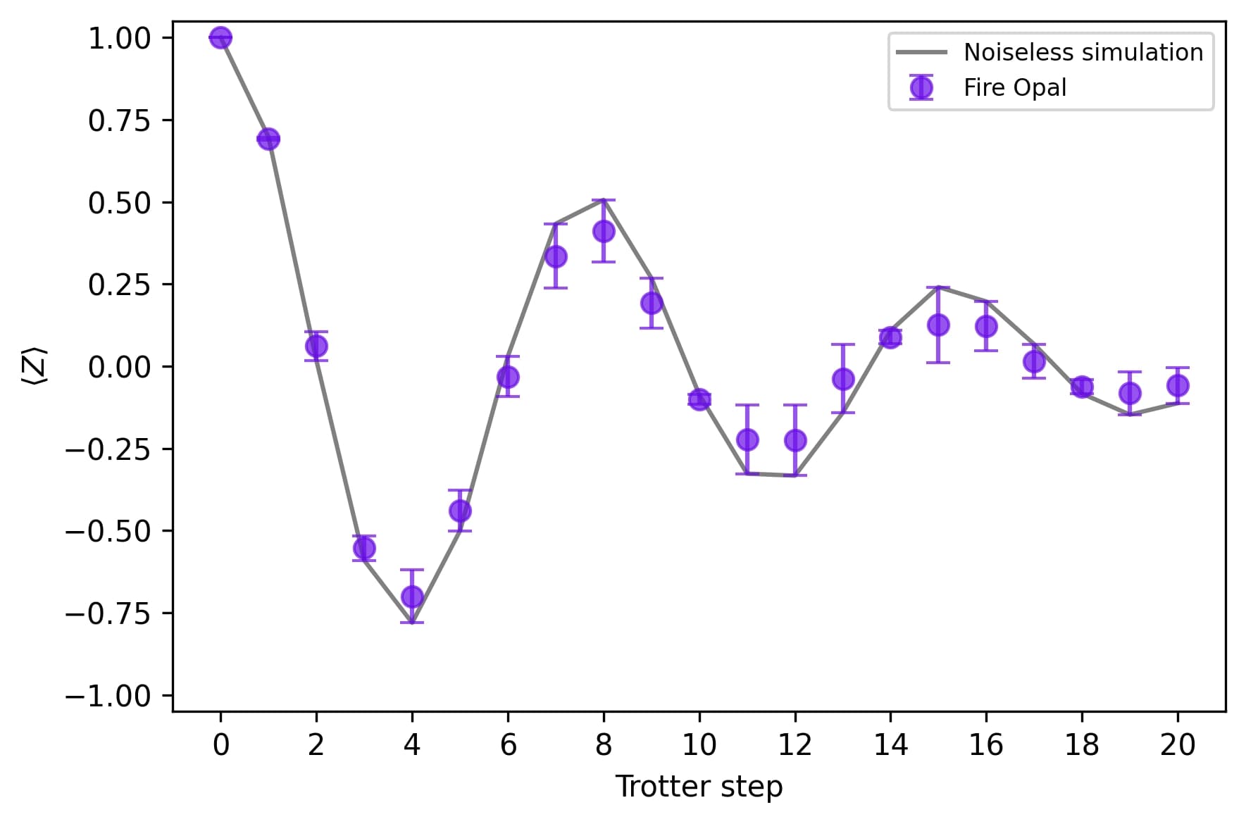
This analysis demonstrates how Fire Opal can be used to calculate the Transverse-field Ising Model. The agreement between simulated and measured results highlights the potential of Fire Opal for capturing key physical behaviors.
from fireopal import print_package_versions

print_package_versions()
| Package | Version |
| --------------------- | ------- |
| Python | 3.12.9 |
| matplotlib | 3.10.1 |
| networkx | 2.8.8 |
| numpy | 1.26.4 |
| qiskit | 1.4.2 |
| qiskit-ibm-runtime | 0.36.1 |
| sympy | 1.13.3 |
| fire-opal | 8.4.1 |
| qctrl-workflow-client | 5.5.0 |
