How to optimize controls using arbitrary basis functions
Create optimized controls from superpositions of basis functions
Boulder Opal exposes a highly flexible optimization engine for general-purpose optimization. The controls can be described in terms of optimizable linear combinations from a set of built in or user-defined basis functions, which can greatly reduce the dimensionality of the optimization search space.
In this user guide, you'll learn how to optimize controls using a Fourier basis, a Hann series basis, or define your own custom basis.
Summary workflow
1. Define basis function for signal composition in the graph
Define the graph that creates a signal as a superposition of basis functions with optimizable coefficients and use it to define your system's Hamiltonian. Traditionally, a randomized Fourier basis is used, although the same technique has also seen success with other bases, for example Slepian functions or Hann functions.
The operations that you can use to build the optimizable signal depend on the basis you want to use:
-
The Boulder Opal optimization engine provides a convenience graph operation,
graph.real_fourier_pwc_signal, for creating optimizable signals in a Fourier basis, suitable for use in a chopped random basis (CRAB) optimization. -
The
signalsattribute of a graph object provides convenience operations to create optimizable signals in a Hann series basis, as either piecewise-constant functions (graph.signals.hann_series_pwc) or as a sampleable function (graph.signals.hann_series_stf). These operations take some potentially optimizablecoefficients, allowing you to easily create an optimizable signal in a Hann series basis. -
You can also define a custom basis using the library of graph operations. In particular, you can create an analytical pulse by creating a node with the
graph.identity_stfoperation, which returns an STF representing the function $f(t) = t$, and then apply arithmetic and mathematical operations to it in order to generate more complex functions.
2. Run graph-based optimization
With the graph object created, you can run an optimization using the boulderopal.run_optimization function, providing the graph, the cost node, and the desired output nodes.
The function returns the results of the optimization.
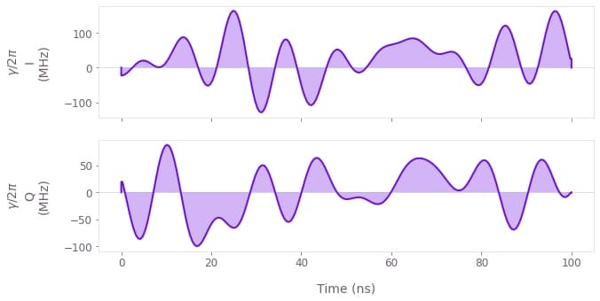
Example: Fourier-basis optimization on a qutrit
In this example, we perform a CRAB optimization (in the Fourier basis) for a robust single qubit Hadamard gate of a qutrit system while minimizing leakage out of the computational subspace, using Hann window functions.
The system is described by the following Hamiltonian: \begin{equation} H(t) = \frac{\chi}{2} (a^\dagger)^2 a^2 + (1+\beta(t)) \left(\gamma(t) a + \gamma^*(t) a^\dagger \right) , \end{equation} where $\chi$ is the anharmonicity, $\gamma(t)$ is a complex time-dependent pulse, $\beta(t)$ is a small, slowly-varying stochastic amplitude noise process, and $a = |0 \rangle \langle 1 | + \sqrt{2} |1 \rangle \langle 2 |$. We will parametrize the optimizable pulses, $\gamma(t)$, as a sum of Fourier components.
import matplotlib.pyplot as plt
import numpy as np

import qctrlvisualizer as qv
import boulderopal as bo
# Define target and projector matrices.
hadamard = np.array([[1.0, 1.0, 0], [1.0, -1.0, 0], [0, 0, np.sqrt(2)]]) / np.sqrt(2)
qubit_projector = np.diag([1.0, 1.0, 0.0])
# Define physical constraints.
chi = 2 * np.pi * -300e6 # Hz
segment_count = 200
duration = 100e-9 # s
gamma_max = 2 * np.pi * 30e6 # Hz
def create_infidelity(graph, gamma):
"""
Define a qutrit Hamiltonian with a drive control given by the input gamma
and calculate the infidelity with respect to the target operation.
"""
# Define standard matrices.
a = graph.annihilation_operator(3)
ada = graph.number_operator(3)
# Create Hamiltonian.
anharmonicity = (ada @ ada - ada) * chi / 2
drive = graph.hermitian_part(2 * gamma * a)
hamiltonian = anharmonicity + drive
# Create target operator in the qubit subspace
target_operator = graph.target(
hadamard.dot(qubit_projector), filter_function_projector=qubit_projector
)
# Create infidelity
infidelity = graph.infidelity_pwc(
hamiltonian=hamiltonian,
target=target_operator,
noise_operators=[drive],
name="infidelity",
)# Number of Fourier terms in superposition.
coefficient_count = 10
# Create optimization graph object.
graph = bo.Graph()
# Create gamma(t) signal in Fourier basis. To demonstrate the full
# flexibility, we show how to use both randomized and optimizable
# basis elements. Elements with fixed frequencies may be chosen too.
gamma_i = graph.real_fourier_pwc_signal(
duration=duration,
segment_count=segment_count,
randomized_frequency_count=coefficient_count,
)
gamma_q = graph.real_fourier_pwc_signal(
duration=duration,
segment_count=segment_count,
optimizable_frequency_count=coefficient_count,
)
gamma = gamma_max * (gamma_i + 1j * gamma_q)
gamma.name = r"$\gamma$"
# Build the rest of the graph.
create_infidelity(graph, gamma)
# Run the optimization
optimization_result = bo.run_optimization(
cost_node_name="infidelity",
output_node_names=[r"$\gamma$"],
graph=graph,
optimization_count=4,
)
print(f"\nOptimized cost: {optimization_result['cost']:.3e}")
qv.plot_controls(optimization_result["output"], smooth=True, polar=False)Your task (action_id="1828723") has started.
Your task (action_id="1828723") has completed.
Optimized cost: 5.799e-07
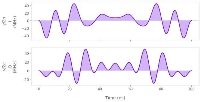
Example: Robust optimization on a qutrit using Hann window functions
In this example, we optimize the same gate as in the previous example, but parametrizing the optimizable pulse using Hann window functions. The signal $\gamma(t) = \gamma_I(t) + i \gamma_Q(t)$ is then expanded as \begin{equation} \gamma_{I(Q)}(t) = \sum_{n=1}^N{\frac{c^{I(Q)}_n}{2} \left[1-\cos\left(\frac{2\pi nt}{\tau_g}\right) \right]}, \end{equation} where $c^{I(Q)}_n$ are the different real-valued coefficients describing the parametrization and $\tau_g$ is the gate duration. This is a good choice for implementation in bandwidth-limited hardware as it is composed of smooth functions that go to zero at the edges.
# Number of terms in Hann superposition.
coefficient_count = 10

# Create optimization graph object.
graph = bo.Graph()

# Define the coefficients of the Hann functions for optimization.
hann_coefficients_i = graph.optimization_variable(
    coefficient_count, lower_bound=-1, upper_bound=1
)
hann_coefficients_q = graph.optimization_variable(
    coefficient_count, lower_bound=-1, upper_bound=1
)
hann_coefficients = gamma_max * (hann_coefficients_i + 1j * hann_coefficients_q)

# Create gamma(t) signal in Hann function basis.
gamma = graph.signals.hann_series_pwc(
    duration=duration,
    segment_count=segment_count,
    coefficients=hann_coefficients,
    name=r"$\gamma$",
)

# Build the rest of the graph.
create_infidelity(graph, gamma)

# Run the optimization and retrieve results.
optimization_result = bo.run_optimization(
    cost_node_name="infidelity",
    output_node_names=r"$\gamma$",
    graph=graph,
    optimization_count=4,
)

print(f"\nOptimized cost: {optimization_result['cost']:.3e}")
qv.plot_controls(optimization_result["output"], smooth=True, polar=False)
Your task (action_id="1828724") has started.
Your task (action_id="1828724") has completed.
Optimized cost: 1.759e-04
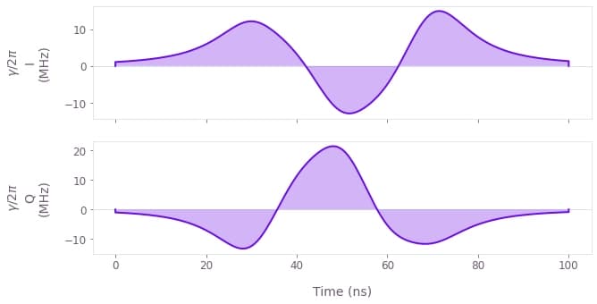
Example: Robust optimization on a qutrit using a custom function superposition
In this example, we optimize the same dynamics as in the previous examples, but with pulses parametrized as a superposition of Lorentz functions. Then, the real and imaginary parts of the optimizable pulse, $\gamma(t) = \gamma_I(t) + i \gamma_Q(t)$, are given by \begin{equation} \gamma_{I(Q)}(t) = \sum_{n=1}^N c^{I(Q)}_n \frac{\sigma^2}{(t - t_n)^2 + \sigma^2} , \end{equation} where $c^{I(Q)}_n$ are the different real-valued coefficients describing the parametrization, $\{t_n\}$ are the centers of the Lorentz functions, and $\sigma$ is their width. This is a good choice for implementation in bandwidth-limited hardware as it is composed of smooth functions that go to zero away from the choice of centers $\{t_n\}$.
Note that you can create a wide variety of analytical functions and superpositions using the different mathematical and arithmetic graph operations.
# Define the function to generate the pulse components.
def custom_optimizable_superposition(graph, duration, coefficient_count, name):
    """
    Create an STF optimizable superposition of Lorentzian functions.

    Parameters
    ----------
    graph : The graph where the signal will belong.
    duration : The duration of the signal.
    coefficient_count : The number of terms in the superposition.
    name : The name of the Tensor node with the optimizable coefficients.

    Returns
    -------
    Stf
        An optimizable superposition of Lorentzian functions.
    """

    # Define optimizable coefficients.
    coefficients = graph.optimization_variable(
        coefficient_count, lower_bound=-1, upper_bound=1, name=name
    )

    # Define Lorentz function parameters.
    width = 0.1 * duration
    centers = np.linspace(0.3, 0.7, coefficient_count) * duration

    # Create Lorentz function superposition.
    time = graph.identity_stf()
    return graph.stf_sum(
        [
            coefficients[index] * width**2 / ((time - center) ** 2 + width**2)
            for index, center in zip(range(coefficient_count), centers)
        ]
    )
# Number of terms in superposition.
coefficient_count = 5
# Create optimization graph object.
graph = bo.Graph()
# Create gamma(t) signal using custom basis.
gamma_i = custom_optimizable_superposition(
graph, duration, coefficient_count, name="coef_i"
)
gamma_q = custom_optimizable_superposition(
graph, duration, coefficient_count, name="coef_q"
)
gamma_stf = gamma_max * (gamma_i + 1j * gamma_q)
# Discretize gamma into PWC.
gamma = graph.discretize_stf(
stf=gamma_stf, duration=duration, segment_count=segment_count, name=r"$\gamma$"
)
# Build the rest of the graph.
create_infidelity(graph, gamma)
# Run the optimization.
optimization_result = bo.run_optimization(
graph=graph,
cost_node_name="infidelity",
output_node_names=[r"$\gamma$", "coef_i", "coef_q"],
optimization_count=4,
)
# Retrieve results and plot optimized pulse.
coefficients_i = gamma_max * optimization_result["output"].pop("coef_i")["value"]
coefficients_q = gamma_max * optimization_result["output"].pop("coef_q")["value"]
print(f"\nOptimized cost: {optimization_result['cost']:.3e}")
print("Optimized coefficients:")
np.set_printoptions(precision=3)
print("\tI:", coefficients_i)
print("\tQ:", coefficients_q)
qv.plot_controls(optimization_result["output"], smooth=True, polar=False)Your task (action_id="1828725") has started.
Your task (action_id="1828725") has completed.
Optimized cost: 8.332e-05
Optimized coefficients:
I: [ 7.927e+07 3.302e+07 -1.078e+08 -5.857e+07 1.337e+08]
Q: [-1.385e+08 7.739e+07 1.745e+08 -9.236e+07 -5.986e+07]