Design robust pulses for dense singlet-triplet qubit arrays

Increasing robustness to charge noise in 2D quantum dot arrays driven by exchange interaction

Boulder Opal provides the functionality to optimize control pulses for dense arrays of semiconductor spin-qubits. The application of control techniques is challenging in these systems, because of two reasons. First, the highly non-linear relation between the control voltages and the exchange interaction is a challenge to gradient-based optimization algorithms and second, the control signals naturally also impose spurious effects on qubits neighboring the target qubit. For this reason the entire qubit array needs to be simulated and we cannot truncate the simulation to one or two qubits.

A recent example for a two-dimensional dense array is the implementation of four singlet-triplet qubits published by X. Zhang et al.. These densely placed singlet-triplet qubits naturally benefit from optimal control techniques, because their Hamiltonian includes an always-on term and driving single qubit rotations leads to spurious coupling with neighboring qubits. At the same time, the system size and non-linearity imposes a challenging control problem.

In this notebook, we will show how such a qubit array can be simulated and how we optimize quantum gates that are robust to charge noise. Thereby, we take into account:

Treatment of the non-linear relation between control voltages and the exchange interaction.
Strong noise dynamics caused by charge noise.
Rescaling control signals for efficient gradient-based optimization.
Pulse filtering to include bandwidth limits of the control electronics.

import numpy as np
import matplotlib.pyplot as plt
from pathlib import Path
from typing import Optional, Union
import copy
import jsonpickle
import time

import boulderopal as bo
import qctrlvisualizer as qv

plt.style.use(qv.get_qctrl_style())


# Read and write helper functions, type independent.
def save_variable(file_name: str, var):
    """
    Save a single variable to a file using jsonpickle.
    """
    with open(file_name, "w") as file:
        encoded_var = jsonpickle.encode(var, unpicklable=True)
        file.write(encoded_var)


def load_variable(file_name: str):
    """
    Load a variable from a file encoded with jsonpickle.
    """
    with open(file_name, "r") as file:
        decoded_var = jsonpickle.decode(file.read())
        return decoded_var


data_folder = Path("resources/")
timestr = time.strftime("%Y%m%d-%H%M%S")
print("Time label for data saved throughout this experiment:" + timestr)

save_files = False
load_files = True
time_label_loading = "20250123-104828"

Time label for data saved throughout this experiment:20250204-143958

Control pulses and degrees of freedom

We simulate a quantum processor architecture consisting of four singlet-triplet qubits that was demonstrated and described by X. Zhang et al. The qubits are formed in an 2×4 quantum dot array.

We label the quantum dots in the following way:

0 - 2 - 4 - 6
|   |   |   |
1 - 3 - 5 - 7

Each vertical pair of quantum dots is tuned into a double quantum dot and is used to define a singlet-triplet qubit resulting in the qubit chain:

Q0 - Q1 - Q2 - Q3

Each adjacent pair of quantum dots $i$ and $j$ is separated by a barrier gate at voltage $B_{ij}$ and the chemical potential of each quantum dot $i$ is controlled by a plunger gate at voltage $P_i$. We define a detuning $\epsilon_{ij}$ as the difference in plunger voltages for neighboring quantum dots, \begin{equation}\epsilon_{ij} = \frac{1}{2}(P_i - P_j) ,\end{equation} and the average plunger voltage \begin{equation}\mu_{ij} = \frac{1}{2}(P_i + P_j) .\end{equation}

We distinguish between intra-qubit detunings that detune two quantum dots forming one qubit e.g. $\epsilon_{01}$ and inter-qubit detuning that detune two quantum dots belonging to different qubits e.g. $\epsilon_{02}$. We use the same terms for barrier voltages and exchange interactions. We keep the average intra-qubit plunger voltages fixed at \begin{equation}\mu_{01} = \mu_{23} = \mu_{45} = \mu_{67} = 0 \end{equation} and define the offsets of the plunger values such that each quantum dot is occupied by a single electron.

We can calculate the inter-qubit detuning of horizontal quantum dot pairs from the intra-qubit detuning of vertical quantum dot pairs. Consider four coupled quantum dots in a rectangle labeled i, j, k, and l:

i - k
|   |
j - l

With the assumption that $\mu_{ij} = \mu_{kl} = 0$ we have \begin{align} \epsilon_{ij} = \frac{1}{2} (P_i - P_j) = P_i = - P_j , \\ \epsilon_{kl} = \frac{1}{2} (P_k - P_l) = P_k = - P_l , \end{align} and therefore \begin{align} \epsilon_{ik} = \frac{1}{2} (P_i - P_k) = \frac{1}{2} (\epsilon_{ij} - \epsilon_{kl}) , \\ \epsilon_{jl} = \frac{1}{2} (P_j - P_l) = \frac{1}{2} (\epsilon_{kl} - \epsilon_{ij}) . \end{align}

In total, this gives the system 14 degrees of freedom including the four intra-qubit detunings and all 10 barrier voltages. We assume that all gates are perfectly virtualized and neglect capacitive crosstalk. The model still includes crosstalk effects that occur due to the detuning inducing a coupling.

# Name generation
def detuning_name(
    dot_1: int, dot_2: int, upscaled: bool = False, filtered: bool = False
):
    prefix = "upscaled " if upscaled else ""
    prefix += "filtered " if filtered else ""
    return prefix + f"$e\_{{{dot\_1}{dot\_2}}}$"


def barrier_name(
    dot_1: int, dot_2: int, upscaled: bool = False, filtered: bool = False
):
    prefix = "upscaled " if upscaled else ""
    prefix += "filtered " if filtered else ""
    return prefix + f"$b\_{{{dot\_1}{dot\_2}}}$"


def exchange_name(dot_1: int, dot_2: int):
    return f"$J\_{{{dot\_1}{dot\_2}}}$"


def effective_exchange_name(qubit_1: int, qubit_2: int):
    return f"$J\_{{{qubit\_1}{qubit\_2}}}^e$"


def calculate_inter_qubit_detunings(voltage_signals: dict[str, bo.graph.Pwc]):
    inter_qubit_detunings = []
    for i in range(3):
        # Upper side of the array
        upper_inter_qubit_e = 0.5 * (
            voltage_signals["intra_qubit_detuning"][i * 1]
            - voltage_signals["intra_qubit_detuning"][i * 1 + 1]
        )
        upper_inter_qubit_e.name = detuning_name(i * 2, i * 2 + 2)
        inter_qubit_detunings.append(upper_inter_qubit_e)

        # Lower side of the array
        lower_inter_qubit_e = -1 * upper_inter_qubit_e
        lower_inter_qubit_e.name = detuning_name(i * 2 + 1, i * 2 + 3)
        inter_qubit_detunings.append(lower_inter_qubit_e)

    voltage_signals["inter_qubit_detuning"] = inter_qubit_detunings
    return voltage_signals

Exchange interaction

The exchange interaction energy between two quantum dots depends approximately exponentially on the detuning and the barrier voltage. We chose to model the exchange interaction with the product ansatz \begin{equation}J = J_0 e^{\vert \epsilon \vert / \epsilon_0} e^{B / B_0}.\end{equation}

# Constants
g_mean = np.asarray([0.33, 0.37, 0.37, 0.35])
bohr_magneton = 5.788e-5  # eV / T
reduced_planck_constant = 4.136e-15 * 1e9  # eV / GHz
mean_magnetic_field = 10e-3  # T
mean_zeeman = (
    2 * np.pi * mean_magnetic_field * bohr_magneton / reduced_planck_constant * g_mean
)

# Exchange interaction
default_j_0 = mean_zeeman  # by tuning of the barrier voltage

# Barrier
b_0 = 10  # mV
b_min = 0  # mV
b_max = 60  # mV
b_shift = -50  # mV. This shift avoids negative values

# Detuning
eps_0 = 1  # mV
eps_min = -4  # mV
eps_max = 4  # mV


def exchange_interaction(
    j_0: float,
    detuning: Union[bo.graph.Tensor, np.ndarray],
    barrier_voltages: Union[bo.graph.Tensor, np.ndarray],
    graph: Optional[bo.Graph] = None,
):
    if graph is None:
        j = (
            j_0
            * np.exp(np.abs(detuning) / eps_0)
            * np.exp((barrier_voltages + b_shift) / b_0)
        )
    else:
        j = (
            j_0
            * graph.exp(graph.abs(detuning) / eps_0)
            * graph.exp((barrier_voltages + b_shift) / b_0)
        )
    return j

Intra-qubit exchange interaction

The intra-qubit exchange interaction can be calculated from the corresponding detuning and barrier voltages \begin{equation}J_{ij} = J_0 e^{\vert \epsilon_{ij} \vert / \epsilon_0} e^{B_{ij} / B_0}. \end{equation}

Inter-qubit coupling

For the two qubit dynamics we also need to consider the inter-qubit exchange interaction that couples horizontal pairs of quantum dots. Consider again four coupled quantum dots in a rectangle labeled i, j, k and l:

i - k
|   |
j - l

Then we can also calculate the exchange interaction in the vertical quantum dot pairs analogously to our treatment of the intra-qubit exchange. We define an effective interaction $J^e$ as average of the inter-qubit exchange interactions \begin{equation}J^e = \frac{1}{2} (J_{ik} + J_{jl}).\end{equation}

def pulses_to_exchange_energies(
    graph: bo.Graph, voltage_signals: dict[str, bo.graph.Pwc]
):
    exchange_energies = dict()
    # Intra-qubit exchange energies.
    intra_qubit_exchange_energies = []
    for i, intra_q_detuning, intra_q_barrier_v in zip(
        range(len(voltage_signals["intra_qubit_detuning"])),
        voltage_signals["intra_qubit_detuning"],
        voltage_signals["intra_qubit_barrier_voltage"],
    ):
        intra_q_exchange_energy = exchange_interaction(
            j_0=default_j_0[i],
            graph=graph,
            detuning=intra_q_detuning,
            barrier_voltages=intra_q_barrier_v,
        )
        intra_q_exchange_energy.name = exchange_name(i * 2, i * 2 + 1)
        intra_qubit_exchange_energies.append(intra_q_exchange_energy)
    exchange_energies["intra_qubit"] = intra_qubit_exchange_energies

    # Inter-qubit exchange energies.
    inter_q_exchange_energies = []
    for i, inter_q_detuning, inter_q_barrier in zip(
        range(len(voltage_signals["inter_qubit_detuning"])),
        voltage_signals["inter_qubit_detuning"],
        voltage_signals["inter_qubit_barrier_voltage"],
    ):
        inter_q_exchange_energy = exchange_interaction(
            j_0=default_j_0[0],
            graph=graph,
            detuning=inter_q_detuning,
            barrier_voltages=inter_q_barrier,
        )
        inter_q_exchange_energy.name = exchange_name(i, i + 2)
        inter_q_exchange_energies.append(inter_q_exchange_energy)
    exchange_energies["inter_qubit"] = inter_q_exchange_energies

    # The effective interaction is given by the average of the inter-qubit
    # exchange energies as described above.
    effective_inter_q_exchange = []
    for i in range(3):
        effective_exchange_energy = 0.5 * (
            exchange_energies["inter_qubit"][i * 2]
            + exchange_energies["inter_qubit"][i * 2 + 1]
        )
        effective_exchange_energy.name = effective_exchange_name(i, i + 1)
        effective_inter_q_exchange.append(effective_exchange_energy)
    exchange_energies["effective_inter_qubit"] = effective_inter_q_exchange

    return exchange_energies

Rescaling

This exponential relation between our control parameters and the energy term in the Hamiltonian is problematic for a gradient-based optimization, because derivatives of small voltage values are exponentially suppressed. We can remedy this issue with a rescaling. We optimize the barrier voltages $B$ on a logarithmic scale and we rescale the detuning $\epsilon$ with the inverse hyperbolic sine. This choice was made, because the hyperbolic sine closely resembles the exponential function of the absolute value, but the hyperbolic sine posesses the advantage of being invertible. We therefore optimize the upscaled voltages $B^\prime$ and $\epsilon^\prime$.

\begin{equation} B^\prime = e^{B} \end{equation} \begin{equation} \epsilon^\prime = \sinh(1.13 \epsilon) \end{equation}

At this point, you might ask why we are not directly optimizing the exchange interaction as it is common practice in many optimization frameworks. Our approach enables the treatment of noise on the voltage level, which makes our model much more accurate. We can take the influence of exponential relationship on the noise dynamics into account whereas other models inaccurately translate quasi-static charge noise into quasi-static noise on the exchange interaction.

def upscaling_barrier(barrier_voltages: np.ndarray) -> np.ndarray:
    return np.exp(barrier_voltages / 10)


def downscaling_barrier(
    graph: bo.Graph, barrier_voltages: bo.graph.Tensor, name=None
) -> bo.graph.Tensor:
    downscaled_b = graph.log(barrier_voltages) * 10
    if name:
        downscaled_b.name = name
    return downscaled_b


def upscaling_detuning(detuning_voltages: np.ndarray) -> np.ndarray:
    return np.sinh(1.13 * detuning_voltages)


def downscaling_detuning(
    graph: bo.Graph, detuning_voltages: bo.graph.Tensor, name=None
) -> bo.graph.Tensor:
    downscaled_eps = (
        graph.log(detuning_voltages + graph.sqrt(graph.pow(detuning_voltages, 2) + 1))
        / 1.13
    )
    if name:
        downscaled_eps.name = name
    return downscaled_eps


def downscale_voltages(graph: bo.Graph, voltage_signals: dict[str, bo.graph.Tensor]):
    """Applies the downscaling to all 14 optimizable control voltages."""
    voltage_signals["intra_qubit_detuning"] = [
        downscaling_detuning(
            graph=graph,
            detuning_voltages=signal,
            name=detuning_name(i * 2, i * 2 + 1, upscaled=False),
        )
        for i, signal in enumerate(voltage_signals["intra_qubit_detuning"])
    ]

    voltage_signals["intra_qubit_barrier_voltage"] = [
        downscaling_barrier(
            graph=graph,
            barrier_voltages=signal,
            name=barrier_name(i * 2, i * 2 + 1, upscaled=False),
        )
        for i, signal in enumerate(voltage_signals["intra_qubit_barrier_voltage"])
    ]

    voltage_signals["inter_qubit_barrier_voltage"] = [
        downscaling_barrier(
            graph=graph,
            barrier_voltages=signal,
            name=barrier_name(i, i + 2, upscaled=False),
        )
        for i, signal in enumerate(voltage_signals["inter_qubit_barrier_voltage"])
    ]

We can verify the resemblence of the rescaling function and the ansatz for the exchange interaction.

# Compare the inverse renormalization to the exchange interaction.
epsilon_range = np.linspace(-5, 5, 100)
plt.plot(
    epsilon_range,
    np.sinh(1.13 * epsilon_range) / 2 / np.pi,
    label="$\sinh(\epsilon)$",
    c=qv.QCTRL_STYLE_COLORS[2],
)
plt.plot(
    epsilon_range,
    np.sign(epsilon_range) * np.exp(np.abs(epsilon_range)) / 2 / np.pi,
    label="$J \, \mathrm{sgn}(\epsilon)$",
    c=qv.QCTRL_STYLE_COLORS[0],
)
plt.xlabel("$\epsilon$ (mV)")
plt.ylabel("$J / 2 \pi$ (GHz)")
plt.legend()
plt.show()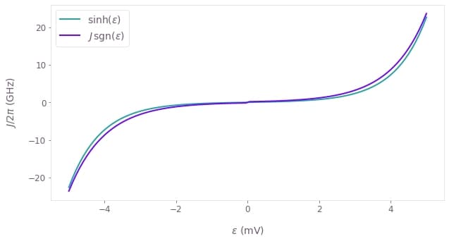

Create control signals

Next we create optimizable control signals.

def create_optimizable_voltages(
    graph: bo.Graph,
    duration: float,
    time_segment_count: int,
    max_detuning=upscaling_detuning(eps_max),
    min_detuning=upscaling_detuning(eps_min),
    max_barrier=upscaling_barrier(b_max),
    min_barrier=upscaling_barrier(b_min),
    upscaled_naming: bool = True,  # mark in names that rescaling is used
):
    # detuning voltages:
    detuning_voltages = []
    for i in range(4):
        optimizable_detuning_voltage = graph.real_optimizable_pwc_signal(
            segment_count=time_segment_count,
            duration=duration,
            maximum=max_detuning,
            minimum=min_detuning,
            name=detuning_name(i * 2, i * 2 + 1, upscaled=upscaled_naming),
        )
        detuning_voltages.append(optimizable_detuning_voltage)

    # barrier voltages:
    intra_q_barrier_voltages = []
    for i in range(4):
        optimizable_intra_q_voltage = graph.real_optimizable_pwc_signal(
            segment_count=time_segment_count,
            duration=duration,
            maximum=max_barrier,
            minimum=min_barrier,
            name=barrier_name(i * 2, i * 2 + 1, upscaled=upscaled_naming),
        )
        intra_q_barrier_voltages.append(optimizable_intra_q_voltage)

    inter_q_barrier_voltages = []
    for i in range(6):
        optimizable_inter_q_voltage = graph.real_optimizable_pwc_signal(
            segment_count=time_segment_count,
            duration=duration,
            maximum=max_barrier,
            minimum=min_barrier,
            initial_values=min_barrier * np.ones(time_segment_count),
            name=barrier_name(i, i + 2, upscaled=upscaled_naming),
        )
        inter_q_barrier_voltages.append(optimizable_inter_q_voltage)

    voltage_signals = {
        "intra_qubit_detuning": detuning_voltages,
        "intra_qubit_barrier_voltage": intra_q_barrier_voltages,
        "inter_qubit_barrier_voltage": inter_q_barrier_voltages,
    }

    return voltage_signals

Convenience functions to create target gates:

def string_to_gate(graph: bo.Graph, string: str):
    if string in ["X", "Y", "Z", "I"]:
        return graph.pauli_matrix(string)
    elif string == "SWAP":
        array_rep = np.diag([1, 0, 0, 1])
        array_rep[1, 2] = 1
        array_rep[2, 1] = 1
        return graph.tensor(array_rep)
    elif string == "CNOT":
        array_rep = np.diag([1, 1, 0, 0])
        array_rep[2, 3] = 1
        array_rep[3, 2] = 1
        return graph.tensor(array_rep)
    else:
        raise ValueError(f"Invalid gate string {string}.")


def string_list_to_gate(graph: bo.Graph, string_list: list[str], name: str = None):
    gate_list = [string_to_gate(graph=graph, string=s) for s in string_list]
    target_gate = graph.kronecker_product_list(gate_list, name=name)
    return target_gate

Charge noise

In this example we focus on charge noise, because it is the most difficult noise source to include. We model the charge noise as quasi-static shifts of the control voltages and all shifts are assumed to vary in their origin and therefore to be uncorrelated. This approach is straight forward and also includes higher-order noise dynamics which can be exponentially amplified in the functional form of the exchange interaction.

Boulder Opal also supports a variety of other noise models. You can find guidance on how to add colored noise or simulate the experiment as an open system in the linked notebooks to include markovian noise.

# Seed the noise trace generation for reproducibility.
noise_seed = 0

# Standard deviation of charge fluctuations on control lines.
std_charge_noise = 0.001  # mV


def add_charge_noise_to_signals(
    graph: bo.Graph,
    noise_sample_count: int,
    sigma: float,
    voltage_signals: dict[str, bo.graph.Pwc],
):
    # We assume that the noise on every physical gate is equal.
    # The standard deviation of the detuning is stronger, because it
    # results from the noise on two plunger gates.
    standard_deviations = {
        "intra_qubit_detuning": np.sqrt(2) * sigma,
        "intra_qubit_barrier_voltage": sigma,
        "inter_qubit_barrier_voltage": sigma,
    }

    noisy_signals = {}
    seed_counter = 0
    for gate_type in voltage_signals:
        noisy_voltage_signals = []
        for voltage_signal in voltage_signals[gate_type]:
            noise_signal = graph.constant_pwc(
                graph.random.normal(
                    shape=[noise_sample_count, 1],
                    mean=0,
                    standard_deviation=standard_deviations[gate_type],
                    seed=noise_seed + seed_counter,
                ),
                duration=sum(voltage_signal.durations),
                batch_dimension_count=1,
            )
            seed_counter += 1
            noisy_voltage_signals.append(noise_signal + voltage_signal)

        noisy_signals[gate_type] = noisy_voltage_signals
    return noisy_signals

Hamiltonian

The considered singlet-triplet qubit is encoded in the singlet state $\ket{S} = (\ket{\uparrow \downarrow} - \ket{\downarrow \uparrow } ) / \sqrt{2}$ and in the lowest-energy triplet state $\ket{T_-} = \ket{\downarrow \downarrow}$. Leakage into the excited triplet states $\ket{T_0}$ and $\ket{T_+}$ is neglected. The Hamiltonian can be formulated with the Pauli operators and a coupling operator that describes the effective 2-qubit interaction.

\begin{equation}\sigma_\mathrm{coup} = \begin{pmatrix} -1 & 0 & 0 & 0 \\ 0 & -1 & 1 & 0 \\ 0 & 1 & -1 & 0 \\ 0 & 0 & 0 & 0 \end{pmatrix}\end{equation}

The coupling operator natively generates a SWAP-like 2-qubit gate that is equivalent to SWAP + iSWAP, but we will show that we can use optimal control techniques to create non-native 2-qubit gates like the CNOT gate.

# coupling operators
coupling_matrix = np.asarray(
    [[-1, 0, 0, 0], [0, -1, 1, 0], [0, 1, -1, 0], [0, 0, 0, 0]]
)


def pauli_and_coupling_operators(graph, qubit_count):
    """Create Pauli and coupling operators for n qubits."""

    if qubit_count == 1:
        embedded_coupling_matrices = []
    elif qubit_count == 2:
        embedded_coupling_matrices = [coupling_matrix]
    else:
        embedded_coupling_matrices = []
        for i in range(qubit_count - 1):
            index_list = [2] * (qubit_count - 2)
            index_list.insert(i, 4)
            embedded_coupling_matrices.append(
                graph.embed_operators(
                    operators=[coupling_matrix, i], dimensions=index_list
                )
            )

    pauli_z_operators = [
        graph.embed_operators(
            operators=[graph.pauli_matrix("Z"), i], dimensions=[2] * qubit_count
        )
        for i in range(qubit_count)
    ]
    pauli_x_operators = [
        graph.embed_operators(
            operators=[graph.pauli_matrix("X"), i], dimensions=[2] * qubit_count
        )
        for i in range(qubit_count)
    ]
    return pauli_x_operators, pauli_z_operators, embedded_coupling_matrices

The Hamiltonian of the system consists of a sum of Hamiltonians describing the dynamics of the singlet-triplet qubits

\begin{equation} H_{ST_-} = \frac{\bar{E}_Z - J}{2} \sigma_z + \frac{\Delta_{ST_-}}{2}\sigma_x\end{equation}

and coupling Hamiltonians for each pair of adjacent qubits

\begin{equation} H_\mathrm{coup} = \frac{J_\mathrm{coup}}{2} \sigma_\mathrm{coup}.\end{equation}

# Always-on X-rotation
delta_st_1f = np.pi / 40  # 2 pi GHz


def build_hamiltonian(graph, exchange_energies):
    (pauli_x_operators, pauli_z_operators, embedded_coupling_matrices) = (
        pauli_and_coupling_operators(graph=graph, qubit_count=4)
    )

    hamiltonian = 0
    # Single qubit terms.
    for i in range(4):
        signal_z = mean_zeeman[i] - exchange_energies["intra_qubit"][i]
        hamiltonian_z = 0.5 * signal_z * pauli_z_operators[i]
        signal_x = delta_st_1f
        hamiltonian_x = 0.5 * signal_x * pauli_x_operators[i]
        hamiltonian += hamiltonian_x + hamiltonian_z

    # Interaction terms.
    for i in range(3):
        hamiltonian += (
            0.5
            * exchange_energies["effective_inter_qubit"][i]
            * embedded_coupling_matrices[i]
        )

    hamiltonian.name = "hamiltonian"
    return hamiltonian

Physical constraints

Our model is an effective model by construction that neglects orbital degrees of freedom and only describes effective spin dynamics. These effective models are derived from single and two-qubit experiments and we need to make further assumptions so that they remain valid in the multi-qubit array. The most important assumption is that for each quantum dot, only a single exchange is driven at a time. In a physical picture, this means that the wave function of each hole stretches only over a single quantum dot or a double quantum dot. We do not form strongly coupled triple quantum dots.

We enforce this assumption and thereby yield physical simulations, by penalizing control pulses that drive two exchange interactions of one dot at the same time. We have adjusted the scaling of the penalty in the overall cost function to balance high fidelity with low overlap simultaneous driving signals on overlapping quantum dot pairs.

def simultaneous_driving_penalty(graph: bo.Graph, exchange_energies):
    penalty = 0
    for i in range(3):
        # product between intra and upper inter
        penalty += graph.sum(
            exchange_energies["intra_qubit"][i].values
            * exchange_energies["inter_qubit"][2 * i].values
        )
        penalty += graph.sum(
            exchange_energies["intra_qubit"][i + 1].values
            * exchange_energies["inter_qubit"][2 * i].values
        )
        # product between intra and lower inter
        penalty += graph.sum(
            exchange_energies["intra_qubit"][i].values
            * exchange_energies["inter_qubit"][2 * i + 1].values
        )
        penalty += graph.sum(
            exchange_energies["intra_qubit"][i + 1].values
            * exchange_energies["inter_qubit"][2 * i + 1].values
        )
    penalty.name = "simultaneous_exchange_penalty"
    return penalty

Bandwidth limitations

In order to create realistic control pulses generated by control electronics with a finite bandwidth, we apply a pulse filtering with a gaussian kernel.

def smooth_voltages(graph: bo.Graph, voltage_signals: dict, segment_count: int):
    kernel = graph.gaussian_convolution_kernel(std=1)

    voltage_signals["intra_qubit_detuning"] = [
        graph.filter_and_resample_pwc(
            pwc=signal,
            kernel=kernel,
            segment_count=segment_count,
            name=detuning_name(i * 2, i * 2 + 1, upscaled=False, filtered=True),
        )
        for i, signal in enumerate(voltage_signals["intra_qubit_detuning"])
    ]

    voltage_signals["intra_qubit_barrier_voltage"] = [
        graph.filter_and_resample_pwc(
            pwc=signal,
            kernel=kernel,
            segment_count=segment_count,
            name=barrier_name(i * 2, i * 2 + 1, upscaled=False, filtered=True),
        )
        for i, signal in enumerate(voltage_signals["intra_qubit_barrier_voltage"])
    ]

    voltage_signals["inter_qubit_barrier_voltage"] = [
        graph.filter_and_resample_pwc(
            pwc=signal,
            kernel=kernel,
            segment_count=segment_count,
            name=barrier_name(i, i + 2, upscaled=False, filtered=True),
        )
        for i, signal in enumerate(voltage_signals["inter_qubit_barrier_voltage"])
    ]

Create Boulder Opal graph

We combine all implemented features in a Boulder Opal graph.

def build_boulder_graph(
    graph: bo.Graph,
    voltage_signals,
    sample_times,
    target_gate_string_list,
    noise_sample_count=1,
    charge_noise_std=std_charge_noise,
    simultaneous_exchange_penalty_factor=1.0,
    rescale_voltages: bool = True,
    filter_voltages: bool = True,
    filtering_segment_count: int = 100,
):
    # Rescale the electronic signals:
    if rescale_voltages:
        downscale_voltages(graph, voltage_signals)

    # Filter the electronic signals:
    if filter_voltages:
        smooth_voltages(graph, voltage_signals, filtering_segment_count)

    # Add Charge noise to signals
    noisy_signals = add_charge_noise_to_signals(
        graph=graph,
        noise_sample_count=noise_sample_count,
        sigma=charge_noise_std,
        voltage_signals=voltage_signals,
    )

    # Calculate inter-qubit detuning
    noisy_signals = calculate_inter_qubit_detunings(voltage_signals=noisy_signals)

    # Calculate exchange energies
    exchange_energies = pulses_to_exchange_energies(
        graph=graph, voltage_signals=noisy_signals
    )

    # Build Hamiltonian
    hamiltonian = build_hamiltonian(graph=graph, exchange_energies=exchange_energies)

    # Calculate the unitary
    propagators = graph.time_evolution_operators_pwc(
        hamiltonian=hamiltonian, sample_times=sample_times, name="propagators"
    )

    # calculate the target gate
    target_gate = string_list_to_gate(
        graph=graph, string_list=target_gate_string_list, name="unitary_target_gate"
    )

    # calculate the infidelity
    infidelity = graph.unitary_infidelity(
        unitary_operator=propagators, target=target_gate, name="infidelity"
    )

    # noise averaged infidelity
    mean_infidelity = graph.sum(
        input_tensor=infidelity / noise_sample_count,
        axis=0,  # the noise batch is the leading dimension
        name="average_infidelity",
    )

    # penalize unphysical situations where a dot has a large overlap
    # with two dots at the same time.
    simultaneous_exchange_penalty = simultaneous_driving_penalty(
        graph=graph, exchange_energies=exchange_energies
    )

    # cost function
    cost_function = (
        mean_infidelity[-1]
        + simultaneous_exchange_penalty_factor * simultaneous_exchange_penalty
    )
    cost_function.name = "cost_function"

    return graph

Convenience functions

To save all control pulses and exchange interactions, we build a full list of names of useful pulse related quantities.

## detuning names
pulse_related_names = []

# filtered pulses
pulse_related_names += [
    detuning_name(i * 2, i * 2 + 1, filtered=True) for i in range(4)
]
pulse_related_names += [barrier_name(i * 2, i * 2 + 1, filtered=True) for i in range(4)]
pulse_related_names += [barrier_name(i, i + 2, filtered=True) for i in range(6)]

## intra_qubit exchange names
pulse_related_names += [exchange_name(i * 2, i * 2 + 1) for i in range(4)]

# effective_exchange
pulse_related_names += [effective_exchange_name(i, i + 1) for i in range(3)]

Optimization of a CNOT gate

We demonstrate the optimization of a CNOT gate, which is not native to the exchange interaction (unlike SWAP-style gates). We show how Boulder Opal can be employed to find control pulses that realize this gate with robustness to charge noise.

For a comparison, we start with the optimization of a control pulse in the absence of charge noise as is standard in most optimal control software packages.

duration = 100
sample_times = [duration]
time_segment_count_pulse = 25
filtering_segment_count = 200
simult_exch_penalty_factor = 0.0005

if not load_files:
    graph_cnot_coh = bo.Graph()
    optimizable_voltages = create_optimizable_voltages(
        graph=graph_cnot_coh,
        duration=duration,
        time_segment_count=time_segment_count_pulse,
    )

    build_boulder_graph(
        graph=graph_cnot_coh,
        voltage_signals=optimizable_voltages,
        sample_times=sample_times,
        target_gate_string_list=["CNOT", "I", "I"],
        noise_sample_count=1,
        charge_noise_std=1e-14,  # practically 0
        rescale_voltages=True,
        simultaneous_exchange_penalty_factor=simult_exch_penalty_factor,
        filter_voltages=True,
        filtering_segment_count=filtering_segment_count,
    )

    result_cnot_coherent = bo.run_optimization(
        graph=graph_cnot_coh,
        cost_node_name="cost_function",
        optimization_count=200,
        output_node_names=pulse_related_names + ["average_infidelity"],
        seed=0,
    )
else:
    filename = data_folder / ("standard_cnot_result_" + time_label_loading)
    result_cnot_coherent = load_variable(filename)
if save_files:
    filename = data_folder / ("standard_cnot_result_" + timestr)
    save_variable(filename, result_cnot_coherent)

if not load_files:
    graph_cnot_noisy = bo.Graph()
    optimizable_voltages = create_optimizable_voltages(
        graph=graph_cnot_noisy,
        duration=duration,
        time_segment_count=time_segment_count_pulse,
    )

    build_boulder_graph(
        graph=graph_cnot_noisy,
        voltage_signals=optimizable_voltages,
        sample_times=sample_times,
        target_gate_string_list=["CNOT", "I", "I"],
        noise_sample_count=80,
        charge_noise_std=1e-3,
        rescale_voltages=True,
        simultaneous_exchange_penalty_factor=simult_exch_penalty_factor,
        filter_voltages=True,
        filtering_segment_count=filtering_segment_count,
    )

    result_cnot_robust = bo.run_optimization(
        graph=graph_cnot_noisy,
        cost_node_name="cost_function",
        optimization_count=1000,
        output_node_names=pulse_related_names + ["average_infidelity"],
        seed=0,
        cost_history_scope="ALL",
    )

else:
    filename = data_folder / ("robust_cnot_result_" + time_label_loading)
    result_cnot_robust = load_variable(filename)

if save_files:
    filename = data_folder / ("robust_cnot_result_" + timestr)
    save_variable(filename, result_cnot_robust)

Next, we compare the noise resilience of both pulses, by averaging over a large number of noise traces to avoid any training bias.

def extract_pulses(result: dict, new_graph: bo.Graph):
    output = result["output"]

    detuning_voltages = [
        new_graph.pwc_signal(
            values=output[detuning_name(i * 2, i * 2 + 1)]["values"],
            duration=np.sum(output[detuning_name(i * 2, i * 2 + 1)]["durations"]),
            name=detuning_name(i * 2, i * 2 + 1),
        )
        for i in range(4)
    ]

    intra_q_barrier_voltages = [
        new_graph.pwc_signal(
            values=output[barrier_name(i * 2, i * 2 + 1)]["values"],
            duration=np.sum(output[barrier_name(i * 2, i * 2 + 1)]["durations"]),
            name=barrier_name(i * 2, i * 2 + 1),
        )
        for i in range(4)
    ]

    inter_q_barrier_voltages = [
        new_graph.pwc_signal(
            values=output[barrier_name(i, i + 2)]["values"],
            duration=np.sum(output[barrier_name(i, i + 2)]["durations"]),
            name=barrier_name(i, i + 2),
        )
        for i in range(6)
    ]

    voltage_signals = {
        "intra_qubit_detuning": detuning_voltages,
        "intra_qubit_barrier_voltage": intra_q_barrier_voltages,
        "inter_qubit_barrier_voltage": inter_q_barrier_voltages,
    }

    return voltage_signals

# Compare the infidelity directly:
chrg_noise_range = np.logspace(-4.5, -2, 60)

standard_pulse_infids = []
robust_pulse_infids = []

for noise_std in chrg_noise_range:
    resimulate_cnot_robust_graph = bo.Graph()
    extracted_pulses_robust = extract_pulses(
        result_cnot_robust, resimulate_cnot_robust_graph
    )
    build_boulder_graph(
        graph=resimulate_cnot_robust_graph,
        voltage_signals=extracted_pulses_robust,
        sample_times=sample_times,
        target_gate_string_list=["CNOT", "I", "I"],
        noise_sample_count=500,
        charge_noise_std=noise_std,
        rescale_voltages=False,
        filter_voltages=True,
        simultaneous_exchange_penalty_factor=0.1,
        filtering_segment_count=filtering_segment_count,
    )
    result_robust_resim_opt = bo.execute_graph(
        graph=resimulate_cnot_robust_graph,
        output_node_names=pulse_related_names + ["average_infidelity", "cost_function"],
    )
    robust_pulse_infids.append(
        result_robust_resim_opt["output"]["average_infidelity"]["value"][-1]
    )

    # Resimulate standard pulse with noise:
    resimulate_cnot_standard_graph = bo.Graph()
    extracted_pulses_coherent = extract_pulses(
        result_cnot_coherent, resimulate_cnot_standard_graph
    )
    build_boulder_graph(
        graph=resimulate_cnot_standard_graph,
        voltage_signals=extracted_pulses_coherent,
        sample_times=sample_times,
        target_gate_string_list=["CNOT", "I", "I"],
        noise_sample_count=500,
        charge_noise_std=noise_std,
        rescale_voltages=False,
        filter_voltages=True,
        simultaneous_exchange_penalty_factor=0.1,
        filtering_segment_count=filtering_segment_count,
    )
    result_coherent_resim_opt = bo.execute_graph(
        graph=resimulate_cnot_standard_graph,
        output_node_names=pulse_related_names + ["average_infidelity", "cost_function"],
    )
    standard_pulse_infids.append(
        result_coherent_resim_opt["output"]["average_infidelity"]["value"][-1]
    )

plt.plot(
    1e3 * chrg_noise_range,
    standard_pulse_infids,
    label="standard",
    c=qv.QCTRL_STYLE_COLORS[1],
)
plt.plot(
    1e3 * chrg_noise_range,
    robust_pulse_infids,
    label="noise robust",
    c=qv.QCTRL_STYLE_COLORS[0],
)
plt.ylabel("Infidelity")
plt.xlabel("Charge noise $\sigma\_\epsilon$ (µV)")
plt.yscale("log")
plt.xscale("log")
plt.legend()
plt.tight_layout()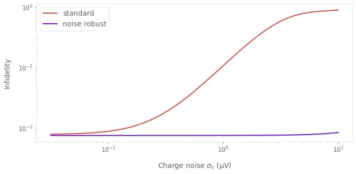

The plot above shows that the robust pulse leads to a strongly suppressed charge noise susceptibility over realistic charge noise ranges, which usually is in the order of a few µV, see for example Dial et al. or Nakajima et al..

Pulse comparison

We can now compare the pulses that were found by the robust and the standard optimization. We start by having a look at the exchange energies in the standard pulse.

def plot_pwc(
    result: dict,
    name_list: list[str],
    title: Optional[str] = None,
    noise_index: Optional[int] = None,
    two_pi_factor: bool = True,
    si_unit_quotient: float = 1e9,
    time_unit_quotient: float = 1e-9,
    unit_symbol: str = "Hz",
):
    controls = {}
    for name in name_list:
        controls[name] = copy.deepcopy(result["output"][name])
        if noise_index is None:
            controls[name]["values"] = np.squeeze(
                si_unit_quotient * controls[name]["values"]
            )
        else:
            controls[name]["values"] = np.squeeze(
                si_unit_quotient * controls[name]["values"][noise_index, ...]
            )

        controls[name]["durations"] = time_unit_quotient * controls[name]["durations"]

    qv.plot_controls(
        controls=controls,
        two_pi_factor=two_pi_factor,
        unit_symbol=unit_symbol,
        smooth=True,
    )
    if title is not None:
        plt.gcf().get_axes()[0].set_title(title)


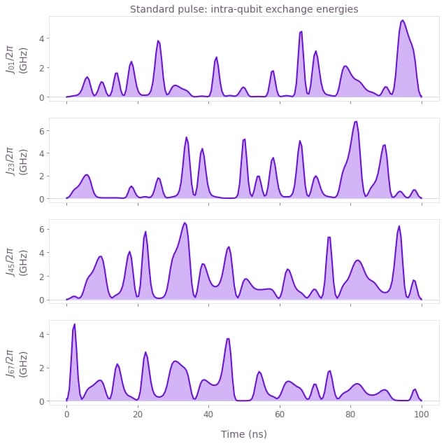
plot_pwc(
    result=result_cnot_coherent,
    name_list=[exchange_name(i * 2, i * 2 + 1) for i in range(4)],
    title="Standard pulse: intra-qubit exchange energies",
)

plot_pwc(
    result=result_cnot_coherent,
    name_list=[effective_exchange_name(i, i + 1) for i in range(3)],
    title="Standard pulse: effective inter-qubit exchange energies",
)

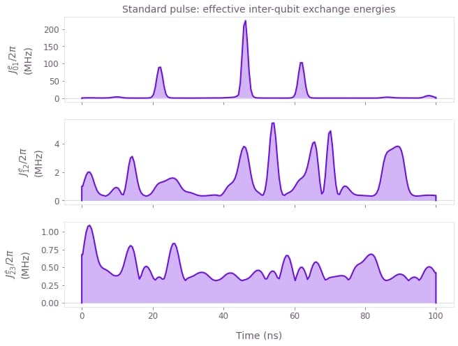
We observe that the intra-qubit exchange interactions on all qubits reach values in the Ghz range. The effective inter-qubit exchange is strong between qubits 0 and 1, where we implement the CNOT gate and small otherwise. (Please note the different units on the Y-axis.)

Next, we look at the exchange values of the robust pulse.

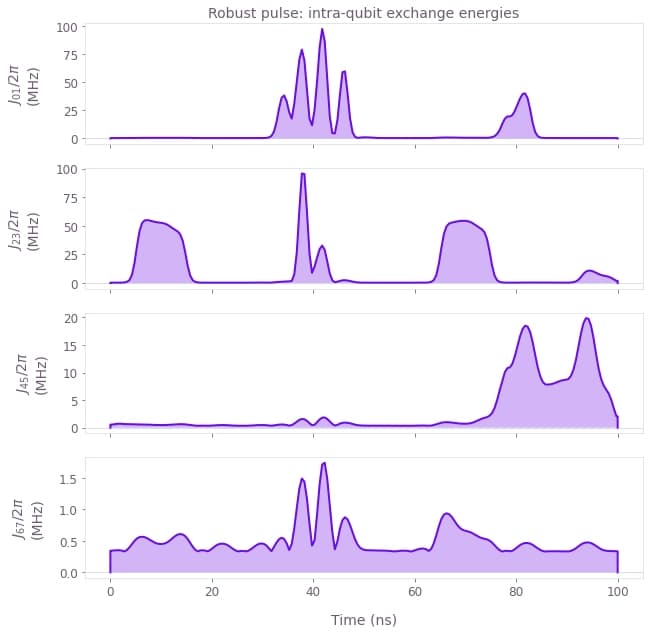
plot_pwc(
    result=result_cnot_robust,
    name_list=[exchange_name(i * 2, i * 2 + 1) for i in range(4)],
    noise_index=0,
    title="Robust pulse: intra-qubit exchange energies",
)

plot_pwc(
    result=result_cnot_robust,
    name_list=[effective_exchange_name(i, i + 1) for i in range(3)],
    noise_index=0,
    title="Robust pulse: effective inter-qubit exchange energies",
)

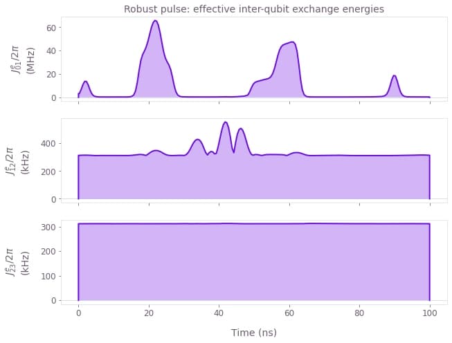
The exchange values are much slower with peak values below 100 MHz. We can observe that a central reason for the noise resilience is the use of lower exchange energies, because the exponential relation between the control pulses and the exchange interaction amplifies noise at higher values. This feature cannot be captured, when a quasi-static noise term is added to the exchange interaction.

We also plot the filtered control pulses for the robust pulse to analyse which gates are primarily used to drive the CNOT gate.

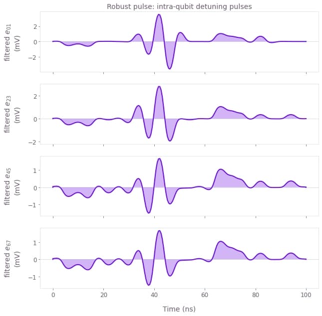
plot_pwc(
    result=result_cnot_robust,
    name_list=[detuning_name(i * 2, i * 2 + 1, filtered=True) for i in range(4)],
    two_pi_factor=False,
    si_unit_quotient=1e-3,
    unit_symbol="V",
    title="Robust pulse: intra-qubit detuning pulses",
)

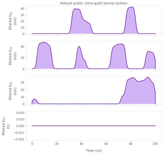
plot_pwc(
    result=result_cnot_robust,
    name_list=[barrier_name(i * 2, i * 2 + 1, filtered=True) for i in range(4)],
    two_pi_factor=False,
    si_unit_quotient=1e-3,
    unit_symbol="V",
    title="Robust pulse: intra-qubit barrier pulses",
)

plot_pwc(
    result=result_cnot_robust,
    name_list=[barrier_name(i, i + 2, filtered=True) for i in range(6)],
    two_pi_factor=False,
    si_unit_quotient=1e-3,
    unit_symbol="V",
    title="Robust pulse: inter-qubit barrier pulses",
)

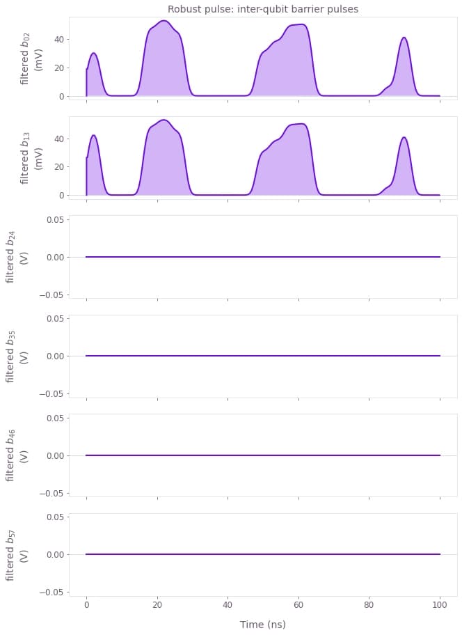
Here, we observe that all control signals are sufficiently smooth. We also note that the interaction is driven more strongly by the barrier voltages. Thereby, our model reproduces the experimental observation that symmetric exchange gates have a smaller susceptibility to charge noise.