Demonstrate SU(3) gates on superconducting hardware
Hamiltonian-agnostic rapid tune-up of an arbitrary unitary on a qutrit
Boulder Opal contains closed-loop optimization tools that enable you to generate optimized controls without requiring a detailed model of your quantum system. This process becomes even simpler and more powerful when software and hardware are seamlessly integrated.
In this application note, we present the entire workflow used to demonstrate the generation, calibration, and benchmark of a high-fidelity SU(3) gate on Lawrence Livermore National Laboratory's superconducting hardware using Boulder Opal integrated with QUA from Quantum Machines. By exploring the multilevel character of transmon qudits, we design gates that go beyond the qubit paradigm. In particular, in our real hardware validation we show that Boulder Opal's closed-loop optimizer provided a pulse with fidelity of 99.8% (an error per gate of 2e-3) for the SU(3) $\pi_{02}$ gate on a transmon qutrit.
We will cover:
- Setting up the experimental runs.
- Defining the appropriate basis functions that parametrize the control pulses to be optimized.
- Setting up a closed-loop optimization using simulated annealing to generate an SU(3) gate.
- Performing the closed-loop optimization experiments in two steps: a coarse optimization followed by an automated fine-tuning of the control pulse.
- Benchmarking the performance of the pulse.
Ultimately we show how to use integrate Boulder Opal's automated closed-loop optimization tools into superconducting circuit experiments, generating high-fidelity optimal controls with minimum knowledge of the system Hamiltonian (for comparison see model-based results).
Imports and initialization
import pickle
from copy import deepcopy

import numpy as np
import matplotlib.pyplot as plt
import qctrlvisualizer as qv

import boulderopal as bo

plt.style.use(qv.get_qctrl_style())

# Choose whether to use saved data or to run experiments.
use_saved_data = True
SU(3) gate in a transmon
In this example, we perform optimization for an SU(3) $\pi_{02}$ gate (that is, $\pi$ rotation in the $|0\rangle - |2\rangle$ subspace while leaving the population in level $|1\rangle$ unchanged) in a qutrit system. The transmon can be approximatelly modeled as a Duffing oscillator and described by the following Hamiltonian:
\begin{align} H(t) = \ \omega_{01} a^\dagger a + \frac{\chi}{2} (a^\dagger)^2 a^2 + \sum_i\left(\gamma_i(t) a + \gamma^*_i(t) a^\dagger \right), \end{align}
where $\omega_{01}$ is the transition frequency from level 0 to 1, $\chi$ is the anharmonicity, $\gamma_i(t)$ are complex time-dependent pulses, and $a = |0 \rangle \langle 1 | + \sqrt{2} |1 \rangle \langle 2 | + ...$ is the annihilation operator.
In this example, we will parametrize the pulse in terms of Hanning window functions which provide a modulation envelope for the two drive frequencies $\omega_{01}$ and $\omega_{12} = \omega_{01} + \chi$:
\begin{align} \gamma(t) = & \ \left( \gamma^{01}_I(t) + i \gamma_Q^{01}(t)\right)e^{i\omega_{01}t} +\left( \gamma^{12}_I(t) + i \gamma_Q^{12}(t)\right)e^{i\omega_{12}t}, \\ \gamma_{I(Q)}(t) = &\sum_{n=1}^N{\frac{c^{I(Q)}_n}{2} \left[1-\cos\left(\frac{2\pi nt}{\tau_g}\right) \right]}, \end{align}
where $c^{I(Q)}_n$ are the different real-valued coefficients describing the parametrization and are distinct for the two drive frequencies while $\tau_g$ is the gate duration. This is a good choice for implementation in bandwidth-limited hardware as it is composed of smooth functions that go to zero at the edges.
Setting up experimental interface
The closed-loop optimization experiment involves sending a pulse to the device, measuring its effect and returning a cost that is fed back to the optimizer. The optimizer then determines a new pulse to be used in the next iteration. This cycle continues until a high-fidelity pulse is found.
The first part of this process is contained in the run_experiments function defined below: It takes a dictionary with the pulse envelopes and returns the cost for optimization.
Channels drive01 and drive12 provide the modulation envelopes for drive frequencies $\omega_{01}$ and $\omega_{12}$ respectively. The corresponding $\pi_{02}$ pulses for the two channels are called Q-CTRL01 and Q-CTRL12. Note that we assume that the initial configuration file was provided and loaded using load_config. We also define an add_pulse_to_config function to add the optimization pulses directly to the QUA config dictionary.
Since our goal is to perform a $[\pi_{02}]$ gate, we define the optimization cost as the population outside level 2 after we apply the pulse to the ground state ($[\pi_{02}]\left|0\right>$).
Note that, for brevity, we do not explicitly show the hardware-specific code. In the cell below, load_config loads and returns a Quantum Machines hardware configuration, and run_quantum_hardware runs the configured experiment returning an array with the final qutrit populations for all requested repetitions.
def add_pulse_to_config(
    pulse_name, channel_name, i_signal, q_signal, config, intermediate_frequency=None
):
    """
    Add a pulse to a QUA config dictionary.

    Parameters
    ----------
    pulse_name : str
        The name of the pulse.
    channel_name : str
        The name of the channel, typically corresponding
        to a specific carrier frequency.
    i_signal : list or np.ndarray
        The I quadrature of the pulse at 1 ns sampling rate.
    q_signal : list or np.ndarray
        The Q quadrature of the pulse at 1 ns sampling rate.
    config : dict
        The main configuration dictionary,
        containing all parameters of the Operator-X (OPX).
    intermediate_frequency : float, optional
        The intermediate frequency of the channel in MHz. If provided, this
        value overrides the intermediate frequency of the `config` dictionary.
        Defaults to None, which means that the original value of the intermediary
        frequency is not modified if it's already present.

    Returns
    -------
    dict
        Updated config dictionary with the new pulses included.

    Raises
    ------
    ValueError
       If the maximum amplitude of I or Q of any pulse is more than 0.49.
    """

    # Copy input config to avoid mutating it.
    config = deepcopy(config)

    if np.max(np.abs(i_signal)) > 0.49 or np.max(np.abs(q_signal)) > 0.49:
        raise ValueError("The maximum amplitude must be below 0.49.")

    if "version" not in config:
        config["version"] = 1

    for key in [
        "controllers",
        "digital_waveforms",
        "integration_weights",
        "mixers",
        "oscillators",
        "waveforms",
        "pulses",
        "elements",
    ]:
        if key not in config:
            config[key] = {}

    if channel_name not in config["elements"]:
        config["elements"][channel_name] = {}
    if "operations" not in config["elements"][channel_name]:
        config["elements"][channel_name]["operations"] = {}
    if intermediate_frequency is not None:
        config["elements"][channel_name][
            "intermediate_frequency"
        ] = intermediate_frequency
    if "intermediate_frequency" not in config["elements"][channel_name]:
        config["elements"][channel_name]["intermediate_frequency"] = None

    config["waveforms"][f"{pulse_name}_I"] = {
        "type": "arbitrary",
        "samples": list(i_signal),
    }
    config["waveforms"][f"{pulse_name}_Q"] = {
        "type": "arbitrary",
        "samples": list(q_signal),
    }
    config["pulses"][pulse_name] = {
        "operation": "control",
        "length": len(i_signal),
        "waveforms": {"I": f"{pulse_name}_I", "Q": f"{pulse_name}_Q"},
    }
    config["elements"][channel_name]["operations"][f"{pulse_name}_op"] = pulse_name

    return config


def run_experiments(parameter_set):
    repetitions = parameter_set["repetitions"]

    # Load a pre-existing config file for Quantum Machines hardware.
    config = load_config()

    # Update pulse to the config.
    config = add_pulse_to_config(
        pulse_name="Q-CTRL01",
        channel_name="drive01",
        i_signal=parameter_set["I_sig01"],
        q_signal=parameter_set["Q_sig01"],
        config=config,
    )
    config = add_pulse_to_config(
        pulse_name="Q-CTRL12",
        channel_name="drive12",
        i_signal=parameter_set["I_sig12"],
        q_signal=parameter_set["Q_sig12"],
        config=config,
    )

    # For brevity, we do not explicitly show the QUA program used to run this experiment.
    populations = run_quantum_hardware(config, repetitions)

    # We aim to maximize the final state 2 population (for all repetitions).
    cost = 1 - np.mean(populations[:, 2])

    return {"cost": cost, "state_population": populations, "repetitions": repetitions}
The next function uses the coefficients of the Hanning functions to construct an array describing the pulse shape with 1ns time step as required by the control hardware
def hanning_function(parameter_set):
    time_step_count = parameter_set["time_step_count"]  # in ns

    # [4, hanning_count] array with all the optimization parameters.
    parameters = np.reshape(parameter_set["parameters"], (4, hanning_count))

    # [time_step_count] array with time samples.
    time_samples = np.arange(time_step_count)  # in ns

    # [hanning_count, 1] array with all frequencies.
    frequencies = (
        2 * np.pi * np.arange(1, hanning_count + 1)[:, None] / (time_step_count - 1)
    )

    # [4, time_step_count] array with all pulse values.
    samples = parameters @ (0.5 * (1 - np.cos(frequencies * time_samples)))

    # Ensure that the final pulses are within [-0.4, 0.4] for all time steps
    # as required by the Quantum Machines control hardware.
    samples = np.clip(samples, -0.4, 0.4)

    I01, Q01, I12, Q12 = samples

    return I01, Q01, I12, Q12
Obtaining the initial test points
After setting up the experimental interface, you need to obtain a set of initial results. You will use these as the initial input for the automated closed-loop optimization algorithm.
The following code initializes the parameters to zero value so that the optimization is started with no prior knowledge of the ideal pulse shape.
# Define the number of test points obtained per run.
test_point_count = 1

# Define number of hanning functions for per channel in the control.
hanning_count = 6
time_step_count = 168

# Initialize parameters.
parameter_set = {
    "time_step_count": time_step_count,
    "repetitions": [1],
    "parameters": [0] * 4 * hanning_count,
}

(
    parameter_set["I_sig01"],
    parameter_set["Q_sig01"],
    parameter_set["I_sig12"],
    parameter_set["Q_sig12"],
) = hanning_function(parameter_set)
Setting up the closed-loop simulated annealing optimizer
Instantiate the simulated annealing process
The simulated annealing hyperparameters, namely temperatures and temperature_cost, respectively control the overall exploration and greediness of the optimizer. More difficult optimization problems typically require higher temperatures because high fidelity controls tend to vary greatly from the initial guesses provided to the optimizer.
In real life problems, determining the optimal choice of temperatures and temperature_cost is generally not feasible or necessary. Some level of searching usually needs to be done on the part of the user. Here, the temperatures have been set to 0.05 after testing temperatures of varying magnitude. Such a search is often easily parallelizable, and heuristically, temperatures 1-2 orders of magnitude smaller than the provided bound tend to be a decent starting point for a search with Hanning window functions. Similar heuristics apply to the temperature_cost, where starting a grid search approximately two orders of magnitude smaller than the range of the cost tends to be a decent starting point. For additional hyperparameter tuning methods, visit the Wikipedia page on hyperparameter optimization.
This section uses the object boulderopal.closed_loop.SimulatedAnnealing to set up an automated closed-loop optimization that uses the simulated annealing (SA) method.
# Define initialization object for the simulated annealing optimizer
bounds = bo.closed_loop.Bounds(np.repeat([[-0.4, 0.4]], hanning_count * 4, axis=0))

optimizer = bo.closed_loop.SimulatedAnnealing(
    bounds=bounds,
    temperatures=[0.05] * hanning_count * 4,
    temperature_cost=0.01,
    seed=0,
)
Now that the optimizer has been set up, we can define the loop that performs the optimization. This is done by calling the function boulderopal.closed_loop.step repeatedly, until the optimizer converges to a low cost (high fidelity) control.
The first call to boulderopal.closed_loop.step should take the optimizer object that is to be used in the optimization. Subsequent calls take the state, a binary object in which the automated closed-loop optimizer stores the current state of the optimization.
def run_optimization(optimizer, parameter_set, tol=0.03):
    # Obtain a set of initial experimental results.
    experiment_results = run_experiments(parameter_set)

    optimization_count = 0
    cost_evolution = [experiment_results["cost"]]
    best_result = experiment_results
    repetitions = parameter_set["repetitions"]

    state = optimizer

    while best_result["cost"] > tol and optimization_count < 400:
        # Organize the experiment results into the proper input format.
        results = bo.closed_loop.Results(
            [parameter_set["parameters"]], [experiment_results["cost"]]
        )

        # Call the automated closed-loop optimizer and obtain the next set of test points.
        optimization_result = bo.closed_loop.step(
            optimizer=state, results=results, test_point_count=test_point_count
        )

        # Print the current best cost.
        print(
            f"Best infidelity after {optimization_count} optimization "
            f"step{'s' if optimization_count > 1 else ''}: "
            f"{best_result['cost']:.3f} "
            f"(current cost: {cost_evolution[optimization_count]:.3f})."
        )

        # Organize the data returned by the automated closed-loop optimizer.
        parameter_set["parameters"] = optimization_result["test_points"][0]
        (
            parameter_set["I_sig01"],
            parameter_set["Q_sig01"],
            parameter_set["I_sig12"],
            parameter_set["Q_sig12"],
        ) = hanning_function(parameter_set)

        state = optimization_result["state"]

        # Obtain experiment results that the automated closed-loop optimizer requested.
        experiment_results = run_experiments(parameter_set)

        # Record the best results after this round of experiments.
        optimization_count += 1
        cost_evolution.append(experiment_results["cost"])

        if cost_evolution[optimization_count] < best_result["cost"]:
            best_result = experiment_results
            best_controls = deepcopy(parameter_set)

    return cost_evolution, best_controls, best_result
Running coarse optimization
With the optimization loop defined, we can now execute the optimization by calling run_optimization. For this first coarse optimization we look at a single application of the gate by setting parameter_set["repetitions"] = [1].
parameter_set["repetitions"] = [1]

if use_saved_data:
    pathname = "resources/"
    filename = "Auto_optim_SWAP_SA_coarse2021_0520_16_00_12data.p"
    data = pickle.load(open(pathname + filename, "rb"))

    cost_evolution = data["cost"]
    best_controls = data["control"][-1]
    best_result = data["best_result"]
else:
    cost_evolution, best_controls, best_result = run_optimization(
        optimizer, parameter_set
    )
qv.plot_controls(
{
r"$\gamma^{01}$": {
"durations": np.ones(time_step_count) * 1e-9,
"values": best_controls["I_sig01"] + 1j * best_controls["Q_sig01"],
},
r"$\gamma^{12}$": {
"durations": np.ones(time_step_count) * 1e-9,
"values": best_controls["I_sig12"] + 1j * best_controls["Q_sig12"],
},
},
polar=False,
unit_symbol="V",
two_pi_factor=False,
smooth=True,
)
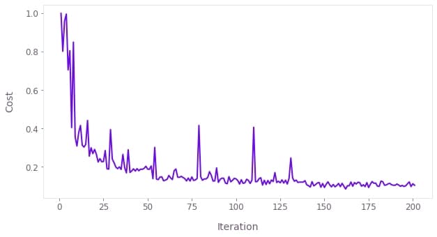
qv.plot_cost_histories(cost_evolution)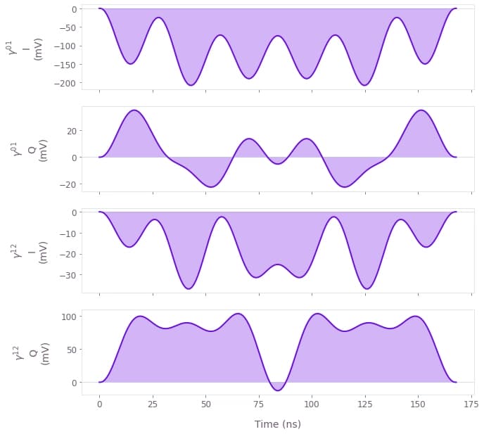
Gate fine-tuning
In order to fine-tune the obtained pulses, we use $4N+1$ gate repetitions ($[\pi_{02}]^{4N+1}\left|0\right>$) for cost evaluation. With this new cost and starting with the best pulse obtained in the coarse optimization above, we run a second, finer, optimization round, by using a simulated annealing optimizer with lower initial temperatures.
if not use_saved_data:
    # Define simulated annealing optimizer.
    optimizer = bo.closed_loop.SimulatedAnnealing(
        bounds=bounds,
        temperatures=[0.003] * hanning_count * 4,
        temperature_cost=0.005,
        seed=0,
    )

    # Run optimization
    parameter_set = deepcopy(best_controls)
    parameter_set["repetitions"] = [1, 5, 9, 13]
    cost_evolution, best_controls, best_result = run_optimization(
        optimizer, parameter_set
    )
Benchmarking the optimized pulse
To benchmark the optimized pulse we measure the qutrit population after applying increasing number of $\pi_{02}$ gates for initial state $\left|0\right>$, $\left|1\right>$, and $\left|2\right>$ respectively. To be concise, we do not show the hardware-specific code for the benchmarking.
if use_saved_data:
    pathname = "resources/"
    filename = "Rep_benchmarking_SWAP_05212021v2.p"
    data = pickle.load(open(pathname + filename, "rb"))
    repetitions = data["rep_vec"]
    populations = data["pop_corr"]
else:
    parameter_set = deepcopy(best_controls)
    repetitions = np.arange(96)
    parameter_set["repetitions"] = repetitions
    populations = run_experiments(parameter_set)
fig, axs = plt.subplots(1, 3, figsize=(15, 5))
fig.suptitle("Population dynamics", y=1.15)
for idx, population in enumerate(populations.values()):
axs[idx].plot(repetitions, population, "-o")
axs[idx].set_title(rf"Initial state $|{idx}\rangle$")
axs[idx].set_xlabel("Repetitions")
axs[0].set_ylabel("Population")
labels = [rf"$|{s}\rangle$" for s in range(3)]
fig.legend(
labels=labels, title="State", loc="center", bbox_to_anchor=(0.5, 1.02), ncol=3
)
plt.show()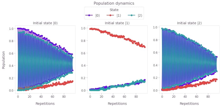
The figure shows the populations of the three qutrit states for different repetitions of $\pi_{02}$ acting on the different basis states. We find no observable leakage into the $\left|1\right>$ state due to the gate as the decay is consistent with the systems's measured T1.
In order to better characterize the pulse fidelity, we apply the error model in H. K. Xu et al.. The fidelity after $m$ repetitions can be described as
\begin{equation}F(m) = A p_\textrm{gate}^m \cos(m\alpha) + B ,\end{equation}
where $p_\textrm{gate}$ is the single-gate fidelity, $\alpha$ is an over-rotation of each gate application, and $A$ and $B$ are SPAM-related parameters. For our results above, we see that the fidelity is primarily coherence limited, and measure a single-gate fidelity of $p_\textrm{gate} = 99.8\%$ and an over-rotation of $\alpha = 0.008$ rad.
