Solving the binary paint shop problem with QAOA
Solve the binary paint shop problem with QAOA using Q-CTRL's performance management on Qiskit Runtime
Quantum approximate optimization algorithm (QAOA) is a popular algorithm that can be applied to a wide range of optimization problems. One such optimization problem that can be solved using QAOA is the binary paint shop problem (BPSP). In this application note, we demonstrate how to solve BPSP using Q-CTRL's natively integrated performance management option within the IBM Quantum platform.
This application note covers the following:
- An introduction to BPSP and its real world applications.
- The derivation of the cost function required to solve BPSP using QAOA.
- A comparison of the performance of the algorithm using Q-CTRL's performance management option versus the Qiskit Runtime default.
1. Introduction
1.1 Problem definition
BPSP is an optimization problem that arises in the context of an automotive paint shop but can also be applied to a variety of industries including printing and textile manufacturing. The paint shop is given a sequence of cars where each car appears exactly twice. A car must be painted with two different colors of paint. The goal is to determine the optimal order in which to paint the cars to minimize the total number of color changes, as the color change procedure is costly in terms of time and resources. This problem is known to be NP-complete and APX-hard. This means finding the optimal solution requires exponential time, and no approximation algorithm exists with a constant approximation ratio. Recent work has demonstrated how QAOA can be used to find solutions for BPSP and, with constant depth, is able to beat classical heuristics in the infinite problem size limit.
Let's denote the set of $n$ cars which should each be painted twice as $\Omega = \{c_0, c_1, ..., c_{n-1}\}$. A single instance of BPSP is given by a sequence $W = (w_0, . . ., w_{2n-1})$ with $w_i \in \Omega$, where each car, $c_i$, appears exactly twice. In practice, this sequence is fixed by contraints posed by the remaining manufacturing processes which are out of the shop's control, such as scheduling due to customer demand. We are given two colors $C = \{0,1\}$ and asked to find a coloring sequence $f = (f_0, ... f_{2n-1})$, where $f_i \in C$, which minimizes the number of color changes between two consecutive cars in the given sequence. Without loss of generality, we will also fix the first color of the first car, $c_0$, to $0$.
1.2 Deriving the cost
To solve this problem using QAOA we start by assigning binary variables to each car where the value of the variable represents the paint color. We denote $0$ as red (🚗) and $1$ as blue (🚙). Then a solution to the problem is given by a paint bitstring, $[x[1], ..., x[n-1]]$, with $x[i] \in C$, which defines the first paint color for car $c_i$. In the paint bitstring encoding, $x[i]=0$ if the car is painted red the first time it appears in the sequence, and blue otherwise. $x[0]$ is removed from the bitstring as car $c_0$ must be assigned to $0$. For every car in our car sequence, $W$, we need to check if the car is being painted for the first or second time and build up the color sequence, $f$, accordingly. Then we can count the number of times the paint color changes for $f$ and find the paint bitstring where this is minimal. In other words, we want to find a paint bitstring which minimizes \begin{equation} \Delta_C = \sum_i |f_i - f_{i+1}|. \end{equation}
For example, say our three-car sequence is equal to $(1, 0, 1, 2, 0, 2)$. The set of possible solutions is $00, 01, 10, 11$, based on the two decision variables $x_1$ and $x_2$ for cars $c_1$ and $c_2$, respectively. The paint bitstring $10$ produces the color sequence $f = ($🚗 🚗 🚙 🚙 🚙 🚗$)$. This corresponds to two paint color changes. We can verify that the solution, $10$, is optimal by calculating the number of color changes for all $2^{n-1}$ possible paint bitstrings. In this three car example, we find two optimal bitstrings, including $10$. $01$, resulting in the color sequence $f = ($🚙 🚗 🚗 🚗 🚙 🚙$)$, is also part of the optimal solution set.
In order to formulate the cost function, counting the number of colour changes, as a polynomial, we will take \begin{equation} |f_i - f_{i+1}| = (f_i - f_{i+1})^2 \end{equation}
The expression must then be converted to a diagonal Qiskit operator representing the multinomial.
2. Imports and initialization
The following section sets up the necessary imports and helper functions.
import matplotlib.pyplot as plt
import numpy as np
import itertools
from sympy import Float, symarray, symbols
from functools import reduce
from qiskit_ibm_runtime import QiskitRuntimeService, Sampler, Session, Options
from qiskit.algorithms.optimizers import COBYLA
from qiskit.algorithms.minimum_eigensolvers import QAOA
from qiskit.opflow import Z
from qiskit.utils import algorithm_globals
import qctrlvisualizer as qv

plt.style.use(qv.get_qctrl_style())
def car_seq_to_color_seq(car_seq, paint_bitstring):
"""
Find the resulting color sequence for the given car sequence and paint bitstring.
"""
painted_once = set()
color_sequence = []
paint_bitstring = paint_bitstring + "0"
for car in car_seq:
if car in painted_once:
color_sequence.append(1 - int(paint_bitstring[-(car + 1)]))
else:
color_sequence.append(int(paint_bitstring[-(car + 1)]))
painted_once.add(car)
return color_sequence
def color_seq_to_emoji_str(color_sequence):
"""
Convert a color sequence to a string of emoji.
"""
emoji_map = {1: "\N{recreational vehicle}", 0: "\N{automobile}"}
emoji_str = ""
for car in color_sequence:
emoji_str += emoji_map[car]
return emoji_str
def plot_histogram(distribution, title=""):
"""
Plot a counts distribution.
"""
bitstrings, counts = zip(
*sorted(distribution.items(), key=lambda item: item[0], reverse=False)
)
plt.figure(figsize=(15, 5))
bars = plt.bar(bitstrings, counts)
plt.xticks(rotation=90, ha="center", fontsize=8)
for index, bitstring in enumerate(bitstrings):
bars[index].set_color("grey")
plt.ylabel("Counts")
plt.title(title)
plt.show()3. Setting up the problem
This section details the problem setup and the definition of the cost function to be minimized.
3.1 Setting up credentials for IBM Quantum services
Initialize an instance of QiskitRuntimeService using the channel_strategy="q-ctrl" to use Q-CTRL's performance management strategy. If you've already saved an account with the channel strategy set, load your saved credentials
You will need to create a new instance of Qiskit Runtime on IBM Cloud to enable the Q-CTRL performance management option. Learn how to set up Q-CTRL performance management on Qiskit Runtime.
# Set credentials - skip if you have already configured Q-CTRL performance management
key = "<IBM Cloud API key>"
instance = "<IBM Cloud CRN>"

QiskitRuntimeService.save_account(
    channel="ibm_cloud",
    channel_strategy="q-ctrl",
    token="<IBM Cloud API key>",
    instance="<IBM Cloud CRN>",
    name="q-ctrl",
    set_as_default=True,
)

# Load the saved credentials
service = QiskitRuntimeService(name="q-ctrl")

# Replace "your_desired_backend" with the name of the device you wish to use.
backend_name = "ibm_algiers"
backend = service.get_backend(backend_name)
3.2 Defining the problem instance
The problem instance will be a randomly generated permutation of 7 cars, each repeated exactly twice.
car_count = 7
car_sequence = np.random.permutation(list(range(car_count)) * 2)
print(f"Randomly generated car sequence to solve for {car_count} cars: {car_sequence}")
Randomly generated car sequence to solve for 7 cars: [4, 2, 6, 3, 3, 4, 1, 1, 0, 5, 0, 6, 2, 5]
3.3 Defining the cost function
Next, specify the cost function as a polynomial cost function represented as a SymPy expr.
def car_sequence_to_cost_multinomial(sequence):
    """
    Generate the multinomial cost function corresponding to the problem.
    """
    variables = symarray("x", len(sequence) // 2)
    painted_once = set()
    color_sequence = []
    variables[0] = 0
    for car in sequence:
        if car in painted_once:
            color_sequence.append(1 - variables[car])
        else:
            color_sequence.append(variables[car])
            painted_once.add(car)
    paint_change_counter = Float(0)
    for c0, c1 in zip(color_sequence, color_sequence[1:]):
        paint_change_counter += (c0 - c1) ** 2
    return paint_change_counter


def cost_multinomial_to_operator(multinomial):
    """
    Derive the operator, or quantum circuit, from the cost function.
    """
    variables = symbols(sorted(str(variable) for variable in multinomial.free_symbols))
    spins = symbols([f"z{i}" for i in range(len(variables))])
    spin_expr = multinomial.subs(list(zip(variables, ((1 - z) / 2 for z in spins))))
    poly = spin_expr.as_poly(spins).as_dict()
    return sum(
        float(coefficient)
        * reduce(lambda a, b: a ^ b, (Z ** (k + 2) for k in monomial))
        for monomial, coefficient in poly.items()
    )


cost_polynomial = car_sequence_to_cost_multinomial(car_sequence)
cost_operator = cost_multinomial_to_operator(cost_polynomial)
print(f"The polynomial cost expression: {cost_polynomial}")
The polynomial cost expression: x_5**2 + x_6**2 + (1 - x_1)**2 + (2*x_1 - 1)**2 + (-x_2 + x_4)**2 + (-x_2 + x_5)**2 + 2*(x_2 - x_6)**2 + (-x_3 + x_4)**2 + (-x_3 + x_6)**2 + (2*x_3 - 1)**2 + (x_5 - 1)**2 + (-x_1 - x_4 + 1)**2
4. Running the algorithm
4.1 Execute with Q-CTRL's performance management
First, execute the problem using the Sampler with Q-CTRL performance management. For Qiskit Runtime instances created with Q-CTRL enabled, an autonomous pipeline works behind-the-scenes to improve the Sampler's algorithmic performance.
algorithm_globals.random_seed = 131242

# Choose a classical optimizer
optimizer = COBYLA()

# Define primitive options and shots
# Q-CTRL performance management is automated and requires no Options config
options = Options()
options.execution.shots = 1024

# Solve the problem using Q-CTRL's performance management behind-the-scenes
# Run the algorithm in a Runtime Session to avoid re-queueing
with Session(service=service, backend=backend):
    sampler = Sampler(options=options)
    qaoa = QAOA(sampler, optimizer, reps=1)
    result = qaoa.compute_minimum_eigenvalue(cost_operator)
dist = {
np.binary_repr(key, car_count - 1)[::-1]: value
for key, value in result.eigenstate.items()
}
plot_histogram(dist)
4.2 Compare results with default Qiskit Runtime settings
Next, you'll switch back to an instance with the default Qiskit Runtime performance to compare results. If you haven't created an Qiskit Runtime instance without Q-CTRL, you'll have to create a new instance of Qiskit Runtime on IBM Cloud. The default Qiskit Runtime settings include error suppression and mitigation too (optimization_level=1, resilience_level=1).
# Set up service with default channel strategy for comparison
key_default = "<IBM Cloud API key>"
instance_without_qctrl = "<IBM Cloud CRN>"
service_without_qctrl = QiskitRuntimeService(
    channel="ibm_cloud", token=key, instance=instance
)
optimizer = COBYLA()
options = Options()
options.execution.shots = 1024
options.optimization_level = 3
options.resilience_level = 0
# Solve the problem using Qiskit Runtime's default settings
with Session(service=service_without_qctrl, backend=backend):
sampler = Sampler(options=options)
qaoa = QAOA(sampler, optimizer, reps=1)
result_default = qaoa.compute_minimum_eigenvalue(cost_operator)dist_default = {
np.binary_repr(key, car_count - 1)[::-1]: value
for key, value in result_default.eigenstate.items()
}
plot_histogram(dist_default)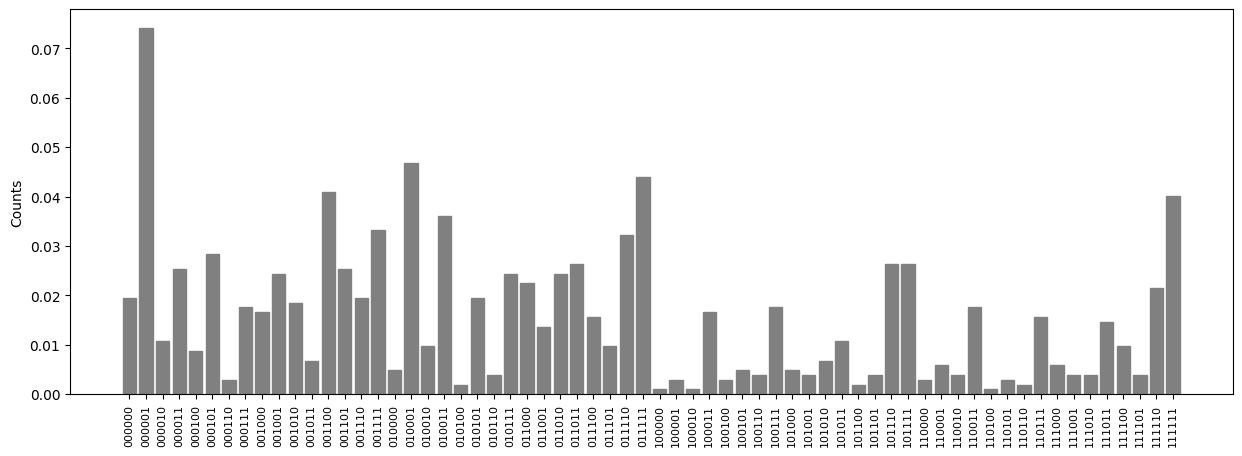
5. Confirming the solution
For a small number of cars, we can manually calculate the number of paint color changes for every possible bitstring, and confirm if the previously found solutions are correct. Because the problem size is relatively small, it's possible to visualize the optimal solution bitstring(s) to confirm that they require the least amount of paint color changes.
brute_force_solution = []
possible_solutions = ["".join(x) for x in itertools.product("01", repeat=car_count - 1)]

# Solve the problem by evaluating all possible bitstrings
for solution_bitstring in possible_solutions:
    paint_change_counter = 0
    color_sequence = car_seq_to_color_seq(car_sequence, solution_bitstring)
    color_sequence
    for c0, c1 in zip(color_sequence, color_sequence[1:]):
        paint_change_counter += np.abs(c0 - c1)
    brute_force_solution.append((solution_bitstring, paint_change_counter))
optimal_change_count = min(brute_force_solution, key=lambda t: t[1])[1]
optimal_bitstrings = [
    bitstring
    for bitstring, count in brute_force_solution
    if count == optimal_change_count
]
# Print and visualize the optimal bitstrings
for bitstring in optimal_bitstrings:
print(
bitstring, color_seq_to_emoji_str(car_seq_to_color_seq(car_sequence, bitstring))
)000001 🚗🚗🚗🚗🚙🚙🚙🚗🚗🚗🚙🚙🚙🚙
Lastly, plot the results histograms on top of one another for a better visual comparision. Check to see if either or both Runtime configurations achieved the correct solution and see which found the correct solution more frequently.
def create_subplot(distribution, ax, title, ylim, solution_color):
    bitstrings, counts = zip(
        *sorted(distribution.items(), key=lambda item: item[0], reverse=False)
    )
    bars = ax.bar(bitstrings, counts)
    ax.set_ylabel("Counts")
    ax.set_ylim(0, ylim)
    ax.set_title(title)
    for index, bitstring in enumerate(bitstrings):
        if bitstring not in optimal_bitstrings:
            bars[index].set_color("grey")
        else:
            bars[index].set_color(solution_color)


fig, axes = plt.subplots(2, 1, figsize=(20, 6), sharex=True)
ylim = max(dist.values()) + 0.1 * max(dist.values())
create_subplot(
    dist, axes[0], "With Q-CTRL", ylim, solution_color=qv.QCTRL_STYLE_COLORS[0]
)
create_subplot(
    dist_default,
    axes[1],
    "Without Q-CTRL",
    ylim,
    solution_color=qv.QCTRL_STYLE_COLORS[1],
)
plt.xticks(rotation=90, ha="center", fontsize=8)
plt.ylabel("Counts")
plt.show()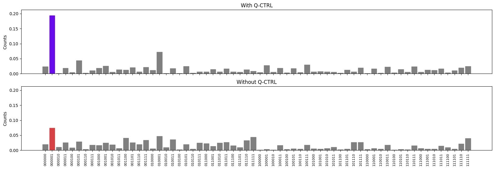
Now you've seen how to solve the binary paint shop problem using Q-CTRL's performance management strategy and compared it to the solution achieve with default Qiskit Runtime settings. Next, try running your own algorithm or application using Q-CTRL Embedded to optimize your execution on IBM Quantum.