Factors that impact Fire Opal's performance improvement
Understanding how to optimize the performance improvement provided by Fire Opal
Quantum algorithms perform orders of magnitude worse than expected when run on real hardware due to the coherence limits of quantum hardware. Fire Opal's automated deterministic error-suppressing workflow bridges this performance gap with zero user configuration and zero QPU overhead. Running quantum circuits with Fire Opal should always provide an advantage over running without. The degree of advantage differs depending on factors outlined in this topic, such as the characteristics of the circuit and the type of algorithm being run.
Circuit depth
Circuit depth is an important property that serves as a measure of complexity. The depth of a quantum circuit signifies how many "layers" of quantum gates, executed in parallel, are required to complete the defined computation. Because quantum gates take time to implement, the depth of a circuit roughly corresponds to the amount of time it takes the quantum computer to execute the circuit. To determine if a quantum circuit can be computed on a given hardware device, circuit depth is a major factor taken into consideration with information about the hardware's tolerance to noise.
Environmental noise causes decoherence to a point where qubits can no longer carry out computation as their states have been too vastly altered by the noise. T1 time is a typical timescale measurement used to characterize the amount of error a quantum computer can tolerate before becoming unusable. While Fire Opal can eliminate or suppress many types of noise, ultimately T1 time is constrained by the hardware device and poses a fundamental limit to the maximum circuit depth that a hardware device can accommodate.
Given the nature of decoherence and its correlation with system size, Fire Opal provides higher success probabilities when executing on shallower circuits. On the other hand, the difference between results with and without Fire Opal is more significant with larger circuits, so long as they don't exceed hardware limitations.
If the circuit depth approaches the T1 limit, Fire Opal will provide a warning in both the execute and validate functions to indicate that you're approaching hardware limits. The benefit that Fire Opal can bring to performance is expected to be less noticeable in these conditions.
If a circuit exceeds T1 limits, the circuit cannot be run on the specified device, and Fire Opal will surface an error. While many hardware providers allow circuits to run, despite them exceeding T1 limits, our intention is to save users from incurring unnecessary QPU usage and costs.
Types of algorithms
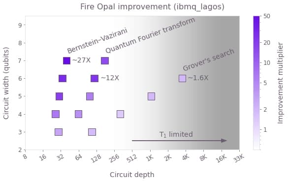
Fire Opal delivers different advantages depending on the algorithm. The performance improvement factor grows with system size until the hardware coherence limits ultimately prevent further execution to be performed. We have benchmarked Fire Opal's error suppression techniques across various algorithms and saw significant improvement in each. To learn more about how Fire Opal improves performance across various algorithms, check out our technical manuscript.
In the previous image shown, we compare three types of algorithms and their performance improvement factor as circuit depth increases. As Grover's search increases in complexity, it also quickly increases in circuit width and depth and becomes limited by the T1 constraints of the hardware. In this type of case, an algorithm will not see as pronounced a performance improvement compared to an algorithm that is naturally more shallow. However, more complex algorithms perform orders of magnitude worse on quantum computers, and Fire Opal makes it possible to achieve useful results that would be otherwise unattainable.
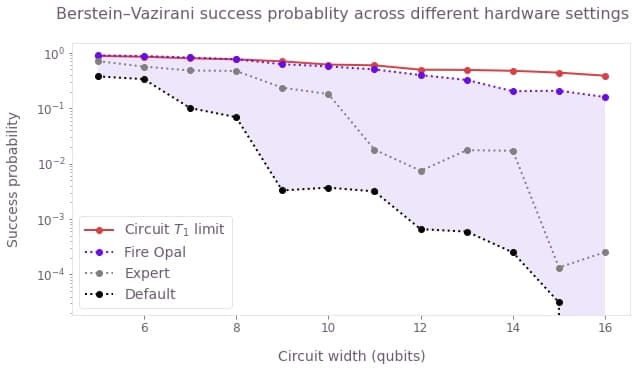
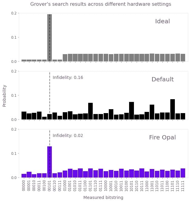
Below are two images showing Fire Opal's results applied to Berstein–Vazirani (top) and Grover's search (bottom). While Fire Opal enabled Berstein–Vazirani to consistently reach near optimal success probabilities, it also provided an 8X improvement to Grover's search and eliminated noise to achieve the correct result.
Expected output distribution
The output of quantum algorithms is a probability distribution of corresponding bitstrings, which can be translated to expected values of possible results. The correct output of the computation of a circuit may be a single one of these bitstrings, multiple bitstrings, or even an uniform distribution of probabilities across the entire range of bitstrings.
As the number of possible results that are expected in the correct outcome increases, it becomes more difficult to extract the correct outputs, and there's a greater likelihood that noise will erase the information used to encode the output. For example, if an algorithm expects a uniform probability over a wide range bitstrings, such as Grover's search, the outcome tends to appear close to a flat distribution. Since noisy computations also produce fairly even distributions, this can make it difficult to perceive the benefits of Fire Opal. For this reason, we recommend ensuring that your anticipated circuit output is distinct from a uniform distribution.
Now that you've learned about how to maximize the benefits of Fire Opal, try it out yourself to see how much you can improve your circuit's success probability.