How to use QuTiP operators in graphs
Incorporate QuTiP objects and programming syntax directly into graphs
It is possible to use Boulder Opal with QuTiP operators.
This is possible in graph execution, where every operator can be replaced by a QuTiP Qobj.
Example: QuTiP operators in a graph-based simulation of a single qubit with leakage
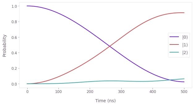
In this example we to simulate the dynamics of a single qubit subject to leakage to an additional level. The resulting qutrit is treated as an oscillator (truncated to three levels) with an anharmonicity of $\chi$, described by the Hamiltonian: \begin{equation} H(t) = \frac{\chi}{2} (a^\dagger)^2 a^2 + \frac{\Omega(t)}{2} a + \frac{\Omega^*(t)}{2} a^\dagger, \end{equation} where $a = |0\rangle \langle 1| + \sqrt{2} |1\rangle \langle 2|$ is the lowering operator and $\Omega(t)$ is a time-dependent Rabi rate.
In the example code below we illustrate how the noise-free infidelity $\mathcal{I}_0$ can be extracted from the coherent simulation results. To do this, we choose as target an X gate between the states $|0\rangle$ and $|1\rangle$. Notice that this target is not unitary in the total Hilbert space, but is still a valid target because it is a partial isometry—in other words, it is unitary in the subspace whose basis is $\{ |0\rangle, |1\rangle \}$.
Note the use of QuTiP to define operators where convenient in defining the relevant graph nodes.
import numpy as np
import matplotlib.pyplot as plt
import qctrlopencontrols as oc
import qctrlvisualizer as qv
import boulderopal as bo

plt.style.use(qv.get_qctrl_style())
# Define system parameters.
chi = 2 * np.pi * 3 * 1e6 # Hz
omega_max = 2 * np.pi * 1e6 # Hz
total_rotation = np.pi
# Define pulse using pulses from Q-CTRL Open Controls.
pulse = oc.new_primitive_control(
rabi_rotation=total_rotation,
azimuthal_angle=0.0,
maximum_rabi_rate=omega_max,
name="primitive",
)
sample_times = np.linspace(0, pulse.duration, 100)
target_operator = np.array([[0, 1, 0], [1, 0, 0], [0, 0, 0]])
try:
import qutip as qt
# Define matrices for the Hamiltonian operators.
a = qt.destroy(3)
n = qt.num(3)
ad2a2 = n * n - n
# Define the target.
target_operation = qt.Qobj(target_operator)
# Define the initial state.
initial_state = qt.basis(3)
graph = bo.Graph()
except ModuleNotFoundError:
graph = bo.Graph()
# Define matrices for the Hamiltonian operators.
a = graph.annihilation_operator(3)
n = graph.number_operator(3)
ad2a2 = n @ n - n
# Define the target.
target_operation = target_operator
# Define the initial state.
initial_state = graph.fock_state(3, 0)[:, None]
pass
# Define the anharmonic term.
anharmonic_drift = 0.5 * chi * ad2a2
# Define Rabi drive term.
rabi_rate = graph.pwc(
durations=pulse.durations,
values=pulse.rabi_rates * np.exp(1j * pulse.azimuthal_angles),
)
rabi_drive = graph.hermitian_part(rabi_rate * a)
hamiltonian = anharmonic_drift + rabi_drive
# Calculate the time-evolution operators.
unitaries = graph.time_evolution_operators_pwc(
hamiltonian=hamiltonian, sample_times=sample_times, name="time_evolution_operators"
)
# Calculate the infidelity.
infidelity = graph.unitary_infidelity(
unitary_operator=unitaries[-1], target=target_operation, name="infidelity"
)
evolved_states = unitaries @ initial_state
evolved_states.name = "evolved_states"
# Run simulation.
graph_result = bo.execute_graph(
graph=graph,
output_node_names=["evolved_states", "infidelity", "time_evolution_operators"],
)
# Extract and print final infidelity.
print(
f"Noise-free infidelity at end: {graph_result['output']['infidelity']['value']:.1e}"
)
# Extract and print final time evolution operator.
print("Time evolution operator at end:")
print(np.round(graph_result["output"]["time_evolution_operators"]["value"][-1], 3))
# Extract and plot state populations.
state_vectors = graph_result["output"]["evolved_states"]["value"]
qv.plot_population_dynamics(
sample_times,
{rf"$|{state}\rangle$": np.abs(state_vectors[:, state]) ** 2 for state in range(3)},
)Your task (action_id="1829175") has completed.
Noise-free infidelity at end: 8.7e-02
Time evolution operator at end:
[[ 0.057-0.145j 0.235-0.926j -0.088+0.235j]
[ 0.235-0.926j -0.067+0.187j -0.193+0.102j]
[-0.088+0.235j -0.193+0.102j -0.825+0.456j]]