Perform narrow-band magnetic-field spectroscopy with NV centers
Using Boulder Opal spectrum reconstruction tools to perform provably optimal leakage-free sensing with spectrally concentrated Slepian pulses
Boulder Opal provides flexible tools for noise characterization and spectroscopy which can be applied to state-of-the art quantum sensors. One key quantum sensor for magnetic fields operates based on nitrogen-vacancy (NV) centers in diamond. The NV center is a spin-1 defect in diamond of significant experimental interest to room temperature quantum magnetometry and nano nuclear magnetic resonance (nano-NMR) spectroscopy, as well as sensing of electric fields, temperature and pressure in exotic environments. In practice, spectroscopy with NV centers typically relies on dynamic-decoupling-pulse sequence-based power spectrum reconstruction methods, such as the Suter–Álvarez (SA) method. Unfortunately, these pulse-based techniques can suffer out-of-band spectral leakage that can lead to signal misidentification.
In this application note, we demonstrate a flexible protocol allowing you to use special controls which suppress spectral leakage. We will cover:
- Analyzing spectral leakage in dynamic decoupling using filter functions
- Designing provably optimal probe controls which suppress spectral leakage
- Using machine learning tools to efficiently perform spectrum reconstruction with any set of controls
We will demonstrate an ability to simply perform magnetic field spectroscopy using NV centers and state-of-the-art machine learning protocols to improve flexibility in measurements, reduce out-of-band sensitivity to background interference to the lowest levels allowed by mathematics, and improve the accuracy of signal reconstruction via minimization of leakage-induced artifacts.
A detailed comparison of Slepian vs SA reconstruction appears in Frey et al. published as Phys. Rev. Applied 14, 024021 (2020).
Imports and initialization
import jsonpickle
import numpy as np
import matplotlib.pyplot as plt

import qctrlvisualizer as qv
import boulderopal as bo

plt.style.use(qv.get_qctrl_style())


def first_order_slepian_based_controls(
    maximum_rabi_rate, duration, segment_count, frequency
):
    """
    Create spectrally concentrated controls derived from first-order Slepian functions.
    """
    times, segment_duration = np.linspace(0, duration, segment_count + 1, retstep=True)
    slepian_envelope = np.kaiser(segment_count + 1, 2 * np.pi)
    total_power = np.sum(np.abs(slepian_envelope * segment_count) ** 2)

    # Cosine shift.
    cos_modulation = np.cos(2 * np.pi * frequency * times)
    slepian = cos_modulation * slepian_envelope

    # Compute the time derivative to obtain dephasing sensitivity.
    slepian = np.diff(slepian)

    # Rescale to maintain power.
    slepian = slepian * np.sqrt(
        total_power / np.sum(np.abs(slepian * segment_count) ** 2)
    )

    # Return control as dict.
    sigma_m = np.array([[0.0, 1.0], [0.0, 0.0]])
    return {
        "operator": sigma_m / 2.0,
        "durations": np.repeat(segment_duration, segment_count),
        "values": maximum_rabi_rate * slepian,
    }


# Read and write helper functions, type independent.
def save_variable(file_name, var):
    """
    Save a single variable to a file using jsonpickle.
    """
    with open(file_name, "w+") as file:
        file.write(jsonpickle.encode(var))


def load_variable(file_name):
    """
    Load a variable from a file encoded with jsonpickle.
    """
    with open(file_name, "r+") as file:
        return jsonpickle.decode(file.read())


data_folder = "./resources/"
Model of the NV center and the magnetic spectrum
In this notebook, we use a single NV center to interrogate a given magnetic field spectrum over a specific window. We begin with a brief look at the relevant NV-center Hamiltonian.
For the purposes of general magnetic field sensing, the ground state of the negatively charged NV center is well described by the following Hamiltonian:
\begin{align} H = DS_z^2 + \gamma_e B_0 S_z + \gamma_eB_1(\cos(\omega t +\phi)S_x + \sin(\omega t +\phi)S_y) + \gamma_e B_{AC} S_z, \end{align}
where $S_{x,y,z}$ are the $S=1$ spin operators and $\gamma_e$ is the gyromagnetic ratio of an electron. The $|\pm1\rangle$ levels are separated from $|0\rangle$ by the zero-field splitting $D=2.87{\rm GHz}$. The background magnetic field $B_0$ is applied along the direction of the NV center quantization axis. The driving field used to control the spin transitions has an amplitude $B_1$, frequency $\omega$, and relative phase $\phi$. Finally, $B_{AC}$ represents the component of the magnetic spectrum fluctuations in the direction of the NV center axis.
In sensing applications, it's typical to run pulse sequences on one of two spin transitions. Setting $\omega=D-\gamma_eB_0$ allows for resonant control of the $|0\rangle \leftrightarrow |-1\rangle$ transition without populating the $|+1\rangle$ level under usual experiment conditions ($D+\gamma_eB_0\gg \gamma_eB_1$). Therefore, this system can be effectively reduced to the following two level Hamiltonian:
\begin{align} H = D\frac{\sigma_z}{2} - \gamma_e B_0 \frac{\sigma_z}{2} + \gamma_eB_1\left(\cos(\omega t +\phi)\frac{\sigma_x}{2} + \sin(\omega t +\phi)\frac{\sigma_y}{2}\right) + \gamma_e B_{AC} \frac{\sigma_z}{2}, \end{align}
where $\sigma_{x,y,z}$ are Pauli matrices. Finally, moving into the rotating frame, the Hamiltonian can be expressed as:
\begin{align} H = \Omega\frac{\sigma_x}{2} + \gamma_e B_{AC} \frac{\sigma_z}{2}, \end{align}
where the driving field has been absorbed into the complex Rabi rate $\Omega= \gamma_e B_1e^{i\phi}$.
We explore the relevance of the control protocol and spectral reconstruction algorithm in reconstructing a synthesized magnetic field spectrum from sensor measurements. The magnetic spectrum we examine is shown below, representing an arbitrary complex environmental landscape containing multiple features—a trait found in various scenarios, from sensing macroscopic objects to nano-NMR.
We interrogate a specific window of the spectrum from $\nu_{\rm min}$ to $\nu_{\rm max}$, here taken to be in the low MHz range. The particular range of the window (for example, whether MHz, kHz, etc.) is arbitrary; however, as we show later, it's essential to note that the spectrum contains features outside of the interrogation window.
# Load power spectrum data.
spectrum_data = load_variable(data_folder + "spectrum_data")
spectrum_frequencies = spectrum_data["spectrum_frequencies"]
spectrum = spectrum_data["spectrum"]


# Interrogation window.
lower_sample_frequency = 2e4
upper_sample_frequency = 2e6
sample_selection = (spectrum_frequencies >= lower_sample_frequency) & (
    spectrum_frequencies <= upper_sample_frequency
)
sample_frequencies = spectrum_frequencies[sample_selection]
sample_spectrum = spectrum[sample_selection]

# Plot spectrum.
fig, ax = plt.subplots(figsize=(15, 5))
ax.plot(spectrum_frequencies / 1e6, spectrum / 1e3, label="Full spectrum", color="gray")
ax.fill_between(spectrum_frequencies / 1e6, spectrum / 1e3, 0, color="lightgray")

ax.plot(sample_frequencies / 1e6, sample_spectrum / 1e3, label="Interrogation window")

ax.set_xlabel("Frequency (MHz)")
ax.set_ylabel("Power density (kWHz$^{-1}$)")
ax.legend()
fig.suptitle("Magnetic field power spectrum")
plt.show()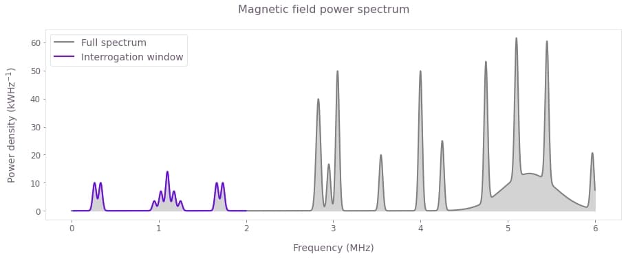
The window we interrogate is highlighted (purple), while the spectrum contains other features outside of it (gray).
Spectrum reconstruction with Suter–Álvarez
Conventional spectroscopy with NV centers often relies on pulse sequences of Carr–Purcell–Meiboom–Gill (CPMG) or XY families, whose filter functions have nontrivial profiles. They are characterized by higher frequency harmonics which interfere with spectrum reconstruction. This issue leads to the appearance of spectrum-dependent artifacts and errors in peak magnitudes.
In this section, we use the SA method to illustrates how out-of-band leakage causes issues with conventional approaches to spectrum reconstruction. The SA technique uses a series of CPMG sequences of fixed duration. It accounts for their harmonics by carefully choosing the sequence order to ensure overlaps between the fundamental and harmonic frequencies of successive sequences. This can be effective in partially mitigating the effects of harmonics in the filter functions, but cannot do so completely and simultaneously adds strict requirements on which measurement sequences may be used.
Filter functions of sequences in conventional spectrum reconstruction approaches
Below we calculate and display the filter functions of all the CPMG sequences used to probe the spectral window of interest. We observe multiple harmonics located outside the interrogation window, a common feature of conventional dynamic decoupling protocols.
# Max Rabi rate of pulses.
maximum_rabi_rate = 2.0 * np.pi * 20 * 1e6

# Duration of CPMG sequences.
duration = 100e-6

# Shot noise.
shot_noise = 1e-4

# Load Suter–Álvarez reconstruction data.
SA_data = load_variable(data_folder + "SA_data")
SA_frequencies = SA_data["frequencies"]
SA_filter_functions = SA_data["filter_functions"]

# Plot spectrum.
fig, ax = plt.subplots(figsize=(15, 5))
fig.suptitle("CPMG filter functions/Power spectrum")
ax.plot(SA_frequencies / 1e6, SA_filter_functions.T, linewidth=0.8)
ax.set_xlabel("Frequency (MHz)")
ax.set_ylabel("Inverse power (W$^{-1}$)")
ax2 = ax.twinx()
ax2.set_ylabel("Spectrum power")
ax2.fill_between(spectrum_frequencies / 1e6, spectrum / 1e3, 0, alpha=0.2, color="k")
plt.show()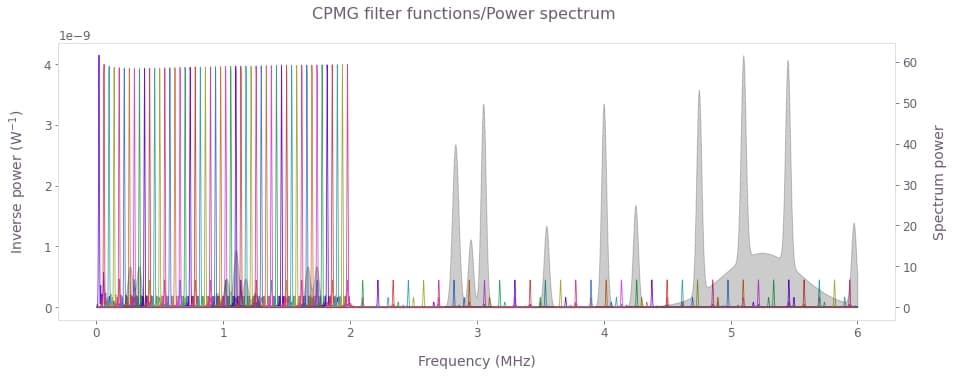
Shown above are the filter functions of CPMG sequences spanning the interrogation window under the SA arrangement. Note that the higher order harmonics cover a significant portion of the spectrum outside the interrogation window. Those harmonics pick up the contributions from the unaccounted spectral components creating errors and artifacts in the reconstruction of the sampled spectrum.
Measurements
The measurements for each of the CPMG sequences would be collected experimentally, however, here they have been simulated using the filter function framework. The probability of finding the NV center in the $m=-1$ state can be estimated as $P_i= \int F^i(\nu)S(\nu)d\nu + \epsilon_m $, where the $F^i(\nu)$ is the filter function of the $i^{th}$ CPMG sequence and $S(\nu)$ is the magnetic power spectrum density. For clarity, the shot noise $\epsilon_m$ is set to be negligible (standard deviation $\sigma=10^{-4}$).
SA_measurements = [m["measurement"] for m in SA_data["measurement_list"]]

fig, ax = plt.subplots(figsize=(15, 5))
ax.plot(SA_measurements, label="", color="k")
ax.set_xlabel("Sequence index")
ax.set_ylabel("Probability")
fig.suptitle("SA measurements")
plt.show()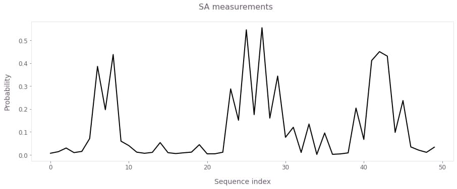
Probability of the $m=-1$ NV state for the index of the CPMG sequence.
Suter–Álvarez reconstruction
The SA algorithm takes in the measurements associated with the CPMG sequences and produces the power spectrum shown below using the method developed by G. A. Álvarez and D. Suter.
SA_reconstructed_frequencies = SA_data["reconstructed_frequencies"]
SA_reconstructed_power = SA_data["reconstructed_power"]

fig, ax = plt.subplots(figsize=(15, 5))
fig.suptitle("Suter–Álvarez power spectrum reconstruction")
ax.plot(sample_frequencies / 1e6, sample_spectrum / 1e3, color="gray")
ax.fill_between(
    sample_frequencies / 1e6,
    sample_spectrum / 1e3,
    0,
    color="lightgray",
    label="True spectrum",
)
ax.plot(
    SA_reconstructed_frequencies / 1e6,
    SA_reconstructed_power / 1e3,
    "-",
    color=qv.QCTRL_STYLE_COLORS[1],
    label="SA reconstructed spectrum",
)
ax.set_xlabel("Frequency (Mhz)")
ax.set_ylabel("Power density (kWHz$^{-1}$)")
ax.legend()
plt.show()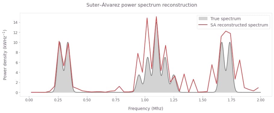
The interrogated section of the spectrum highlights discrepancies between the true spectrum (gray) and the spectrum reconstructed with the Suter–Álvarez technique (red). We observe that in comparison to the plot of measurements in the section above, the SA technique managed to correct the artifacts caused by harmonic within the interrogation window as seen around the feature on the left. However, SA misses some of the features of the real spectrum while simultaneously adding spurious ones due to the effects of out-of-band harmonic leakage, as seen in features in the middle and right. In this example, the amount of power that has leaked into the interrogation window is around $67\%$.
Spectrum reconstruction with Boulder Opal
We perform spectrum reconstruction using an alternate method based on narrowband Slepian functions. An overview of the general method is available the Boulder Opal noise characterization user guide.
Slepian-based controls
Here we use first order Slepians to derive spectrally concentrated pulses that probe specific frequencies free of higher-order harmonics. These pulses will have the same duration as the CPMG sequences above, however, they'll be composed of the time derivative of the continuous Slepian waveform modulated by the frequencies you want to interrogate in order to ensure sensitivity in the $\sigma_{z}$ quadrature associated with sensing of a magnetic field.
Below is the array of Slepian-based controls; each constitutes a variable width envelope combined with a modulation which shifts the band-center of the control's response.
# Points at which to probe the frequency window.
sample_point_count = 100
slepian_frequencies = np.linspace(
    lower_sample_frequency, upper_sample_frequency, sample_point_count
)

# Set up gradually varying Rabi rates to make filter function amplitudes constant.
slepian_rabi_rate_0 = 2 * np.pi * 15e3
slepian_rabi_rates = slepian_rabi_rate_0 * slepian_frequencies / slepian_frequencies[0]

# Number of segments the Slepian pulse is discretized into.
segment_count = 4000

# Generate the array of Slepian-based controls.
slepian_based_controls = [
    first_order_slepian_based_controls(rabi_rate, duration, segment_count, frequency)
    for frequency, rabi_rate in zip(slepian_frequencies, slepian_rabi_rates)
]
# Plot the Slepian-based controls.
indices = [9, 19, 79]
f1, f2, f3 = np.array([slepian_frequencies[idx] for idx in indices]) / 1e6
qv.plot_controls(
{r"$\Omega\_{ %s }$" % idx: slepian_based_controls[idx] for idx in indices},
smooth=True,
)
plt.suptitle(f"Slepian-based pulses for sampling frequencies {f1}, {f2}, and {f3} MHz")
plt.show()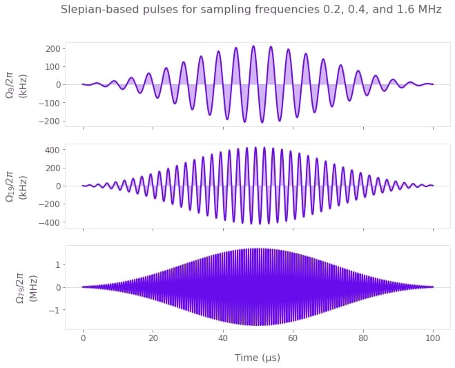
Above, we present a selection of the Slepian-based pulses. The frequency that each control is set to probe is controlled by modulation of the Slepian envelope. An advantage of these controls is that you can keep them at a fixed duration while continuously sweeping across the spectrum.
Next we compute the filter functions of the Slepian-based pulses. There is an option to use pre-computed results for faster evaluation. Note that the performance of the filter function calculations benefits from eager execution mode.
use_saved_data = True

if use_saved_data:
    slepian_filter_functions = load_variable(data_folder + "slepian_filter_functions")
else:
    graph = bo.Graph()
    names = [f"filter_function_{idx}" for idx in range(len(slepian_based_controls))]
    for control, name in zip(slepian_based_controls, names):
        drive_term = graph.hermitian_part(
            graph.pwc(durations=control["durations"], values=control["values"])
            * (2 * control["operator"])
        )
        drift_term = graph.constant_pwc_operator(
            duration=duration, operator=graph.pauli_matrix("Z") / 2
        )

        control_hamiltonian = drive_term + drift_term

        frequency_domain_noise_operators = graph.frequency_domain_noise_operator(
            control_hamiltonian=control_hamiltonian,
            noise_operator=drift_term,
            frequencies=spectrum_frequencies,
            sample_count=2000,
        )

        # Take the y-axis projection in the control frame
        # as the y component contributes to the measurements, that is,
        # N_y(f) = 𝜎_y ⟨𝜎_y, N(f)⟩.
        cf_axis = graph.pauli_matrix("Y")[None]
        slepian_frequency_domain_control_operators_y_proj = (
            graph.trace(frequency_domain_noise_operators @ cf_axis)[..., None, None]
            * cf_axis
        )

        # Compute the filter functions in the subspace.
        slepian_filter_function = graph.sum(
            graph.abs(slepian_frequency_domain_control_operators_y_proj) ** 2 / 2,
            axis=(1, 2),
            name=name,
        )

    result = bo.execute_graph(
        graph=graph, output_node_names=names, execution_mode="EAGER"
    )
    slepian_filter_functions = np.stack(
        [result["output"][name]["value"] for name in names]
    )
    save_variable(data_folder + "slepian_filter_functions", slepian_filter_functions)
# Plot spectrum.
fig, ax = plt.subplots(figsize=(15, 5))
ax.plot(spectrum_frequencies / 1e6, slepian_filter_functions.T, linewidth=0.8)
ax.set_xlabel("Frequency (MHz)")
ax.set_ylabel("Inverse power (W$^{-1}$)")
fig.suptitle("Slepian filter functions/Power spectrum")
ax2 = ax.twinx()
ax2.fill_between(spectrum_frequencies / 1e6, spectrum / 1e3, 0, alpha=0.25, color="k")
ax2.set_ylabel("Spectrum power")
plt.show()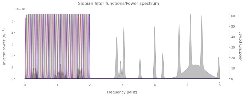
As shown above, the Slepian-based pulses have a highly concentrated frequency response enabling interrogation of an arbitrary section of the spectrum without out-of-band leakage. The reconstruction procedure we use here can accommodate various sampling strategies—there are no strict requirements on the form of the sequences used as the reconstruction algorithm in Boulder Opal is much more flexible than the original SA technique. With the selected controls and their respective bandwidths we form an array of overlapping samples in a manner that ensures high-resolution sampling of the interrogation window.
Measurements
The measurements for Slepian-based controls are calculated using the filter function framework as described before; in experimental applications these would be derived directly from measurements on hardware.
# Simulated measurements.
shot_noise = 1e-4

slepian_measurements = []
for ff in slepian_filter_functions:
    measurement = np.trapz(ff * spectrum, x=spectrum_frequencies)
    # Shot noise.
    measurement += np.random.default_rng().normal(0.0, shot_noise, 1)
    slepian_measurements.append(np.abs(measurement)[0])
slepian_measurements = np.array(slepian_measurements)

# Plot measurements.
fig, ax = plt.subplots(figsize=(15, 5))
ax.plot(slepian_frequencies / 1e6, slepian_measurements, color="k")
ax.set_xlabel("Frequency (MHz)")
ax.set_ylabel(r"Probability")
fig.suptitle("Slepian measurements")
plt.show()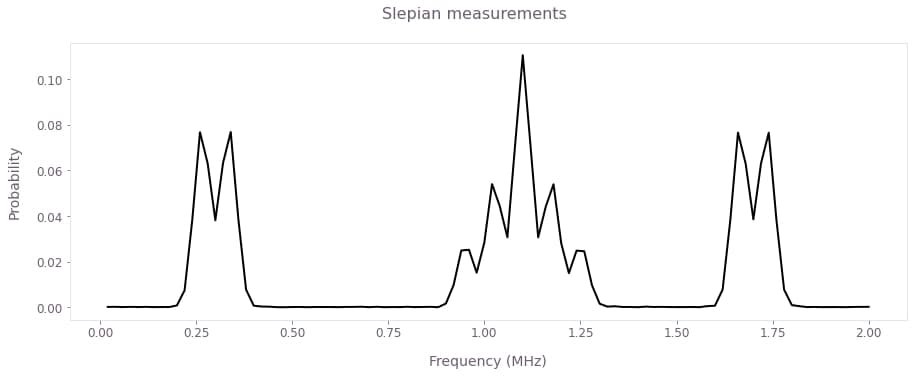
The raw measurements obtained using the Slepian-based controls are free of artifacts and already reflect the spectrum closely.
Reconstruct the power spectrum with high accuracy
To capture the full frequency response of your controls, the mapping $\mathbf{M}$ between the measurements $\mathbf{P}$ and the power spectrum $\mathbf{S}$ will be based on the filter function framework. The measurement associated with the $i^{th}$ control pulse can be expressed in discretized form as follows: \begin{align} P_i = \sum_{j=1}^N F^i_j S_j \Delta \nu, \end{align} where the filter function of the control $F^i$ and the spectrum $\mathbf{S}$ are sampled with spectral resolution $\Delta \nu = (\nu_{\rm max}-\nu_{\rm min})/N$. Therefore, scaling the filter functions of the selected controls by $\Delta \nu$ and arranging them in a matrix enables construction of $\mathbf{M}$, such that $\mathbf{P} = \mathbf{M}\mathbf{S}$.
In the final step, we invert the mapping $M$ in order to reconstruct the interrogated section of the spectrum $\mathbf{S} = \mathbf{M^{-1}}\mathbf{P}$. Boulder Opal offers two different efficient inversion procedures powered by TensorFlow, and purpose built with spectral reconstruction in mind. They are based on single value decomposition (SVD) and convex optimization (CVX).
Both methods provide parameter free estimation needed for reconstruction of unknown power spectrum densities. The SVD procedure offers high numerical efficiency for smooth, slow-varying spectra, but may introduce unphysical oscillations in the reconstructed spectrum when these conditions are not met. By enforcing strict positivity, the CVX inversion procedure provides superior results for spectra exhibiting abrupt changes and rapid variations, as in the current example. For this reason, we use the CVX procedure in the reconstruction implementation below.
For more details and a comparison between the reconstruction methods, refer to Ball et al., as well as our noise spectrum reconstruction user guide.
# Configure CVX reconstruction method.
cvx_method = bo.noise_reconstruction.ConvexOptimization(
    power_density_lower_bound=0,
    power_density_upper_bound=1e9,
    regularization_hyperparameter=1e-12,
)
# Perform reconstruction with CVX.
sample_filter_functions = slepian_filter_functions[:, sample_selection]
filter_functions = [
    bo.noise_reconstruction.FilterFunction(sample_frequencies, filter_function)
    for filter_function in sample_filter_functions
]
noise_reconstruction_result = bo.noise_reconstruction.reconstruct(
    filter_functions=[filter_functions],
    infidelities=slepian_measurements,
    method=cvx_method,
)

# Extract reconstructed PSD.
spectrum = noise_reconstruction_result["output"][0]
Your task (action_id="1828084") has started.
Your task (action_id="1828084") has completed.
# Plot reconstructed spectrum.
fig, ax = plt.subplots(figsize=(15, 5))
ax.fill_between(
    spectrum["frequencies"] / 1e6,
    spectrum["psd"] / 1e3,
    0,
    color="lightgray",
    label="True spectrum",
)
ax.plot(
    spectrum["frequencies"] / 1e6,
    spectrum["psd"] / 1e3,
    "-",
    label="Reconstructed spectrum",
)
ax.set_xlabel("Frequency")
ax.set_ylabel("Power density (kWHz$^{-1}$)")
ax.legend()
fig.suptitle("Power spectrum reconstruction with Boulder Opal")
plt.show()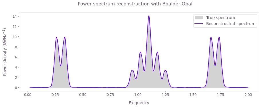
By basing the reconstruction on detailed spectral response of your controls, Boulder Opal provides full flexibility in designing customized controls and sampling strategies to probe any noise spectrum. The plot above shows a highly accurate power spectrum reconstruction using Boulder Opal tools for the case where concentrated, harmonic-free Slepian controls are used.
