Improve Z2 state generation by 3X on QuEra's Aquila QPU
Deployment of Boulder Opal optimal pulses to increase the fidelity of state preparation in a cold atom cloud quantum computer hardware
In this application note, we demonstrate how Boulder Opal can be used to improve the performance of state preparation problems on a neutral atom quantum processor. We illustrate the interoperability with QuEra's Bloqade package by numerically verifying the expected pulse performance using Bloqade simulations. In particular, we demonstrate that a Boulder Opal optimized pulse can improve preparation fidelity of an antiferromagnetic phase in neutral atoms, also known as a Z2 phase, by a factor of 3 compared to a benchmark pulse. These results are demonstrated through a deployment of the optimized pulse on the QuEra Aquila QPU via Amazon Braket.
To run this notebook, we assume that you have installed Julia, Bloqade and JuliaCall to allow Boulder Opal to interface with the Bloqade simulation tools. Experiments are run directly using the Amazon Braket Python SDK and do not require the packages above.
Imports and setup
import sys
import numpy as np
import matplotlib.pyplot as plt
import boulderopal as bo

import qctrlvisualizer as qv

from braket.ahs.atom_arrangement import AtomArrangement
from quera_ahs_utils.plotting import plot_avg_density
from quera_ahs_utils.drive import get_drive

from functools import partial

plt.style.use(qv.get_qctrl_style())
This notebook includes additional code in the resources directory which are used to support interoperability with Bloqade. In the next cell we import functions from this code which are required for the application note. The code can be found in resources/quera_z2_optimization.py should you wish to examine or modify it.
sys.path.append("resources")

import quera_z2_optimization as qctrl_quera

plot_avg_density = partial(plot_avg_density, cmap=qctrl_quera.density_cmap)
Optimize pulse to prepare a Z2 state
This section uses Boulder Opal to optimize the performance of a pulse to prepare the Z2 state, which we will compare with a benchmark pulse similar to the ones used in QuEra's Bloqade tutorial. The system used to optimize the pulse is a small 1D chain with 7 atomic qubits, enabling efficient modelling and optimization with Boulder Opal.
First we define the function to perform the optimization with Boulder Opal. This function takes parameters for maximum Rabi rate, detuning, duration of the pulse, length of atomic chain and interatomic separation to use for the optimization. The final optimization result is returned as a dictionary. Note that the optimization enforces smoothing of the pulse by filtering the control signal as described in this user guide.
# Rydberg blockade coefficient in rad µm^6 / s
BLOCKADE_COEFFICIENT = 5420441.132650757e6


def optimize_z2_pulse(
    omega_max,
    delta_max,
    duration,
    kernel_width,
    atom_count,
    atom_separation,
    optimization_count=4,
    iteration_count=2000,
    segment_count=128,
):
    graph = bo.Graph()

    # Define system operators.
    sigma_z = graph.pauli_matrix("Z")

    interaction_strength = BLOCKADE_COEFFICIENT / atom_separation**6
    drive_operator, detuning_operator, blockade_operator = qctrl_quera.get_operators(
        atom_count, interaction_strength
    )

    # Set up optimizable variables for omega and delta.
    optimization_variable_count = 11
    amplitude_input, detuning_input = qctrl_quera.add_pwc_signals_to_graph(
        graph,
        optimization_variable_count=optimization_variable_count,
        omega_max=omega_max,
        delta_max=delta_max,
        duration=duration,
    )

    # Filter the signals.
    omega, delta = qctrl_quera.envelope_and_filter_graph(
        graph,
        segment_count,
        amplitude_input,
        detuning_input,
        kernel_width,
        0.7,
        duration,
    )
    omega.name = "amplitude"
    delta.name = "detuning"

    # Create Hamiltonian.
    drive_term = omega * drive_operator
    delta_term = -delta * detuning_operator

    hamiltonian = drive_term + delta_term + blockade_operator

    initial_state = graph.fock_state(2**atom_count, 0)

    unitary_operator = graph.time_evolution_operators_pwc(
        hamiltonian=hamiltonian, sample_times=[duration]
    )
    final_state = unitary_operator[-1] @ initial_state[:, None]
    final_state = final_state[:, 0]
    final_state.name = "state"

    sigma_zs = [
        graph.embed_operators((sigma_z, 1), [2**i, 2, 2 ** (atom_count - i - 1)])
        for i in range(atom_count)
    ]
    adjacent_spin_parity = [
        sigma_zs[i] @ sigma_zs[i + 1] for i in range(atom_count - 1)
    ]
    adjacent_spin_parity = graph.sum(adjacent_spin_parity, axis=0)
    adjacent_parity_cost = graph.real(
        graph.expectation_value(final_state, adjacent_spin_parity)
    )
    adjacent_parity_cost.name = "adjacent_parity_cost"

    output_node_names = ["amplitude", "detuning", "state", "adjacent_parity_cost"]
    cost_node_name = "adjacent_parity_cost"

    return bo.run_optimization(
        graph=graph,
        output_node_names=output_node_names,
        cost_node_name=cost_node_name,
        optimization_count=optimization_count,
    )
Then either run the optimization for the desired parameters, or load a pre-computed optimization result by setting create_new_pulse = False:
create_new_pulse = False

atom_separation = 6.1  # µm
num_atoms_opt = 7
num_atoms_sim = 13

register_sim = AtomArrangement()
# Offset registers for plotting.
register_offset = AtomArrangement()
register_offset_2 = AtomArrangement()
for i in range(num_atoms_sim):
    y = np.round(i * atom_separation * 1e-6, 7)
    register_sim.add([0.0, y])
    register_offset.add([1.0e-6, y])
    register_offset_2.add([2.0e-6, y])


# Set maximum Rabi rate and detuning for the pulse.
omega_max = 2.5e6 * 2 * np.pi  # rad/s
duration = 1.5e-6  # s
delta_max = 9e6 * 2 * np.pi  # rad/s

filter_kernel_width = 1.35e-7

if create_new_pulse:
    result = optimize_z2_pulse(
        omega_max,
        delta_max,
        duration,
        filter_kernel_width,
        num_atoms_opt,
        atom_separation,
    )
else:
    # Load the saved optimization result.
    result = qctrl_quera.load_result("resources/quera_z2_optimized_pulse.json")

print(f"Cost: {result['cost']:.3e}")
Cost: -5.998e+00
Compare Bloqade simulations of benchmark pulse and the optimized pulse
Here we demonstrate that the optimized pulse prepares the Z2 state with high fidelity, and that the high-performance state preparation generalizes to longer chains of atoms than the original 7-atom optimization target system. We simulate the performance of the optimized pulse on a 13-atom chain.
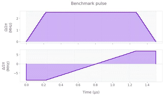
First we plot the controls for both the Boulder Opal optimized pulse and the benchmark pulse for comparison. We use a linear "ramp/soak" pulse for the benchmark, which is commonly used in these types of state preparation problems. See, for example, the Bloqade documentation page on adiabatic state preparation which uses similar pulse profiles.
benchmark_pulse = qctrl_quera.load_result("resources/z2_benchmark_pulse_1p50_us.json")

omega_values = benchmark_pulse["amplitude"] / 1e6
delta_values = benchmark_pulse["detuning"] / 1e6
durations = benchmark_pulse["durations"] * 1e6

qv.plot_controls(
    {
        r"$\Omega$": result["output"]["amplitude"],
        r"$\Delta$": result["output"]["detuning"],
    }
)
plt.suptitle("Q-CTRL pulse")

qv.plot_controls(
    {
        r"$\Omega$": {"values": omega_values * 1e6, "durations": durations * 1e-6},
        r"$\Delta$": {"values": delta_values * 1e6, "durations": durations * 1e-6},
    }
)
plt.suptitle("Benchmark pulse")

plt.show()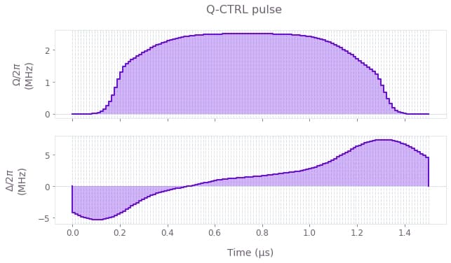
Then, we simulate the evolution of both pulses on the 13-atom system using Bloqade:
omega_qctrl, delta_qctrl = qctrl_quera.qctrl_pulse_to_bloqade(result)
omega_benchmark = qctrl_quera.bloqade_pwc(omega_values, durations)
delta_benchmark = qctrl_quera.bloqade_pwc(delta_values, durations)

atoms = qctrl_quera.chain_lattice(num_atoms_sim, atom_separation)

sim_hamiltonian_qctrl = qctrl_quera.bloqade_two_level_hamiltonian(
    atoms, omega_r=omega_qctrl, delta_r=delta_qctrl
)
sim_hamiltonian_benchmark = qctrl_quera.bloqade_two_level_hamiltonian(
    atoms, omega_r=omega_benchmark, delta_r=delta_benchmark
)

final_state_qctrl = qctrl_quera.bloqade_simulate_nq(
    num_atoms_sim, sim_hamiltonian_qctrl, duration * 1e6
)
final_state_benchmark = qctrl_quera.bloqade_simulate_nq(
    num_atoms_sim, sim_hamiltonian_benchmark, duration * 1e6
)

final_density_qctrl = qctrl_quera.average_rydberg_density(
    final_state_qctrl, num_atoms_sim
)
final_density_benchmark = qctrl_quera.average_rydberg_density(
    final_state_benchmark, num_atoms_sim
)
Finally we can analyze the results. First we compare the final Rydberg density (probability of each atom being measured in the Rydberg state), noting that the target values alternate between 0 and 1 on adjacent atoms. The result of our optimized pulse is much closer to this target, especially towards the center of the chain. We can see this improvement by plotting the Rydberg density - the alternating pattern is much clearer for the Q-CTRL pulse.
ideal_rydberg_density = np.array([1.0, 0.0] * (num_atoms_sim // 2) + [1.0])

fig, ax = plt.subplots(1, 1, figsize=(10, 5))

plot_avg_density(final_density_benchmark, register_sim, custom_axes=ax)
plot_avg_density(final_density_qctrl, register_offset, custom_axes=ax)
plot_avg_density(ideal_rydberg_density, register_offset_2, custom_axes=ax)

plt.xlim(-0.5, 2.5)

ax.set_xticks([0.0, 1.0, 2.0])
ax.set_xlabel("")
ax.set_xticklabels(["Benchmark", "Q-CTRL", "Target state"])

fig.axes[-2].remove()
fig.axes[-2].remove()

fig.tight_layout()

plt.show()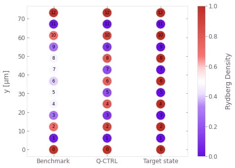
Another way of analyzing the problem is to look at the probability of measuring each bitstring after the state preparation. Here we plot this measurement probability for the 10 most probable bitstrings, for both the benchmark and optimized pulses. The bitstring corresponding to the target state is marked in red:
benchmark_sim_pmf = np.abs(final_state_benchmark[:, 0]) ** 2
qctrl_sim_pmf = np.abs(final_state_qctrl[:, 0]) ** 2

fig, ax = plt.subplots(1, 1, figsize=(10, 5))

qctrl_quera.plot_bitstring_comparison(
    qctrl_sim_pmf, benchmark_sim_pmf, ax, "Optimized pulse", "Benchmark pulse"
)

plt.legend()
plt.title("Simulated bitstring probability")

plt.show()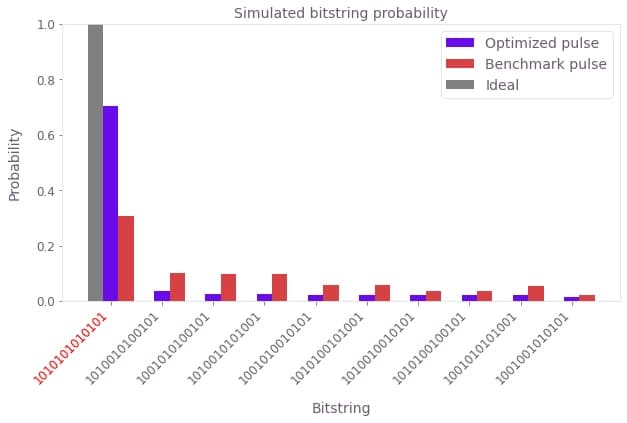
The simulation shows that the Q-CTRL pulse improves the state preparation fidelity, defined as the probability of measuring the bitstring corresponding to the target state, from 30% to over 70%. This represents a performance improvement of over 2X for a pulse of the same duration and comparable laser power.
Hardware demonstration
We will now demonstrate deployment of a pulse developed using the above optimization procedure to QuEra's Aquila QPU via Amazon Braket, showing the performance of the optimization on real hardware. Results from an example deployment are available for the saved result provided with this application note. If you choose to optimize a new pulse by setting create_new_pulse = True above, then you will need to provide an AWS CLI profile name with access to Amazon Braket and credits to use Aquila in order to run the hardware demonstration for your new optimized pulse. This is specified using the profile_name variable below. Note that submitting jobs to the Aquila QPU carries an associated cost and requires you to install the Amazon Braket Python SDK. If you do not wish to incur these costs you can instead load the results of the example deployment.
if create_new_pulse:
    # Imports required to test Q-CTRL pulse on hardware via Amazon Braket.

    from boto3 import Session
    from braket.aws import AwsSession, AwsDevice
    from braket.ahs.analog_hamiltonian_simulation import AnalogHamiltonianSimulation

    profile_name = ""

    boto_sess = Session(profile_name=profile_name, region_name="us-east-1")
    aws_session = AwsSession(boto_session=boto_sess)

    register_deploy = register_sim

    qpu = AwsDevice(
        "arn:aws:braket:us-east-1::device/qpu/quera/Aquila", aws_session=aws_session
    )

    omega_pwc = result["output"]["amplitude"]
    delta_pwc = result["output"]["detuning"]

    (time_points, amplitude_values, detuning_values) = (
        qctrl_quera.pwc_to_piecewise_linear(omega_pwc, delta_pwc)
    )

    phase_values = np.zeros_like(time_points)

    drive = get_drive(time_points, amplitude_values, detuning_values, phase_values)

    qpu_program = AnalogHamiltonianSimulation(
        register=register_deploy, hamiltonian=drive
    )
    task = qpu.run(qpu_program, shots=1000)
    qctrl_shots = task.result()
    qctrl_quera.save_braket_result(
        "resources/quera_z2_optimized_hardware_result", qctrl_shots, drop_bad_shots=True
    )
qctrl_results = 1 - qctrl_quera.load_braket_result(
"resources/quera_z2_optimized_hardware_result"
)Now we plot the probability of measuring each bitstring for the optimized and benchmark pulses deployed on Aquila. The target state bitstring is highlighted in red and the light gray bar represents the ideal outcome.
def shots_to_pmf(shots):
    """
    Convert raw measurements to a probability of each bitstring.
    """
    num_qubits = shots.shape[1]
    counts = np.zeros(2**num_qubits, dtype="int")
    for shot in shots:
        # Convert bits to an integer to index the counting array
        shot_as_int = int(np.sum(2 ** np.arange(num_qubits)[::-1] * shot))
        counts[shot_as_int] += 1
    pmf = counts / shots.shape[0]
    return pmf


benchmark_deployment_results = 1 - qctrl_quera.load_braket_result(
    "resources/z2_benchmark_pulse_hardware_result"
)

benchmark_deployment_pmf = shots_to_pmf(benchmark_deployment_results)
qctrl_deployment_pmf = shots_to_pmf(qctrl_results)

fig, ax = plt.subplots(1, 2, figsize=(15, 5))

qctrl_quera.plot_bitstring_comparison(qctrl_sim_pmf, benchmark_sim_pmf, ax[0])

qctrl_quera.plot_bitstring_comparison(
    qctrl_deployment_pmf,
    benchmark_deployment_pmf,
    ax[1],
    "Optimized pulse",
    "Benchmark pulse",
)

ax[0].set_title("Simulated")
ax[1].set_title("Hardware deployment")

ax[1].legend()

plt.suptitle("Bitstring probabilities")

plt.show()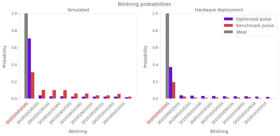
We see that the benchmark pulse deployment prepares the target state with low probability, whereas the Boulder Opal optimized pulse gives a much higher target state probability of around 40%. The probability of measuring the target bitstring on hardware is still lower than that predicted in simulation for the optimized pulse. This is largely due to the significant (8%) readout error associated with the Rydberg state on the device. We have prepared a probability distribution of bitstrings from an example pulse developed using this same optimization procedure, after application of Q-CTRL's measurement error mitigation techniques used in Fire Opal. Measurement mitigation accounts for the readout errors by correcting the measured probability distribution. In the following cell we plot this mitigated probability distribution for comparison with the benchmark pulse:
qctrl_mitigated_pmf = np.loadtxt("resources/z2_optimised_pulse_mitigated_pmf")

fig, ax = plt.subplots(1, 1, figsize=(10, 5))
qctrl_quera.plot_bitstring_comparison(
    qctrl_mitigated_pmf,
    benchmark_deployment_pmf,
    ax,
    "Optimized pulse + measurement mitigation",
    "Benchmark pulse",
)
plt.legend()

plt.title("Bitstring probabilities from hardware")

plt.show()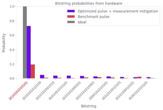
We see that the measurement mitigation procedure boosts the target state preparation fidelity to over 70%, in agreement with the performance level shown in the simulations.
