Generate highly-entangled states in large Rydberg-atom arrays
Generating high-fidelity GHZ states using Boulder Opal pulses
Boulder Opal offers a flexible optimization engine that can be applied to either unitary operations or state preparation in order to enhance quantum computer performance. This capability is highly relevant to recent work demonstrating the potential of trapped Rydberg atoms for applications in quantum computing. One key challenge is state initialization, where complex multipartite states must be engineered from an array of atoms initialized in the ground state.
In this application note, we demonstrate optimized pulses that generate GHZ states for an array of multiple atoms with high fidelity. We will demonstrate:
- Optimizing controls using sparse Hamiltonians and Krylov subspaces.
- Simulating system dynamics.
- Validating performance as a function of atomic array-length.
- Simulating the effects of spontaneous emission on system dynamics using the jump-based trajectory method.
Ultimately this work demonstrates how optimal control techniques can be used to efficiently prepare complex multipartite systems and increase operation speed in Rydberg-atom experiments.
Imports and initialization
import time
import numpy as np
import scipy
import jsonpickle
import jsonpickle.ext.numpy as jsonpickle_numpy
import matplotlib as mpl
import matplotlib.pyplot as plt
import qctrlvisualizer as qv

import boulderopal as bo

jsonpickle_numpy.register_handlers()
plt.style.use(qv.get_qctrl_style())
bo.cloud.set_verbosity("QUIET")
# Total time for the evolution.
duration = 1.1e-6 # s
# Interaction strength.
default_interaction_strength = 24.0e6 * (2 * np.pi) # Hz
# Helper functions.
def create_target_state(qubit_count, level_count=2):
# Indices of states |0101...⟩ and |10101...⟩.
idx_even = sum(2**n for n in range(0, qubit_count, 2))
idx_odd = sum(2**n for n in range(1, qubit_count, 2))
target_state = np.zeros([level_count**qubit_count])
target_state[[idx_even, idx_odd]] = 1.0 / np.sqrt(2.0)
return target_state
def get_recommended_k(
qubit_count,
segment_count,
level_count=2,
interaction_strength=default_interaction_strength,
):
"""
Calculate the appropriate Krylov subspace dimension (k)
required for an integration, from the Hamiltonian with the
largest spectral range.
"""
# Calculate terms and put together the full Hamiltonian.
H_omega, H_delta, H_fixed = get_rydberg_hamiltonian_terms(
qubit_count, level_count=level_count, interaction_strength=interaction_strength
)
graph = bo.Graph()
maximal_range_hamiltonian = (
omega_max * H_omega - delta_range * H_delta + H_fixed
).tocoo()
# Calculate spectral range.
spectral_range = graph.spectral_range(operator=maximal_range_hamiltonian)
# Calculate the appropriate Krylov subspace dimension k.
graph.estimated_krylov_subspace_dimension_lanczos(
spectral_range=spectral_range,
error_tolerance=1e-6,
duration=duration,
maximum_segment_duration=duration / segment_count,
name="k",
)
result = bo.execute_graph(graph, "k")
return result["output"]["k"]["value"]
# Read and write helper functions, type independent.
def save_variable(file_name, var):
"""
Save a single variable to a file using jsonpickle.
"""
with open(file_name, "w+") as file:
file.write(jsonpickle.encode(var))
def load_variable(file_name):
"""
Load a variable from a file encoded with jsonpickle.
"""
with open(file_name, "r+") as file:
return jsonpickle.decode(file.read())Generating GHZ states using Boulder Opal pulses
Characterizing the dynamics of the Rydberg system
Consider a chain of $N$ atoms, each one modeled as a qubit, with $|0\rangle$ representing the ground state and $|1\rangle$ representing a Rydberg state. The total Hamiltonian of the system, as described by A. Omran et al., is given by \begin{equation} H = \frac{\Omega(t)}{2} \sum_{i=1}^N \sigma_x^{(i)} - \sum_{i=1}^N (\Delta(t) +\delta_i) n_i + \sum_{i<j}^N \frac{V}{\vert i-j \vert^6}n_i n_j , \end{equation} with $\sigma_x^{(i)} = \vert 0 \rangle \langle 1 \vert_i + \vert 1 \rangle \langle 0 \vert_i$, and $n_i = \vert 1\rangle\langle 1 \vert_i$.
The fixed system parameters are the interaction strength between excited atoms, $V= 2\pi \times 24$ MHz, and the local energy shifts $\delta_i$, \begin{align} \delta_i &= 2 \pi \times \begin{cases} - 4.5 \ \mathrm{MHz} \quad \mathrm{for} \ i=1,N \\ 0 \quad \mathrm{otherwise} \end{cases} \qquad \mathrm{for} \ N \leq 8 , \\ \delta_i &= 2 \pi \times \begin{cases} - 6.0 \ \mathrm{MHz} \quad \mathrm{for} \ i=1,N \\ - 1.5 \ \mathrm{MHz} \quad \mathrm{for} \ i=4,N-3 \\ 0 \quad \mathrm{otherwise} \end{cases} \qquad \mathrm{for} \ N > 8 . \end{align}
The control parameters are the effective coupling strength to the Rydberg state and the detuning, $\Omega(t)$ and $\Delta(t)$ respectively. These can be manipulated during the system evolution, which is specified to take place over a total time $T = 1.1$ µs. For convenience, the Hamiltonian terms can be grouped as follows: \begin{equation} H = \Omega(t) H_\Omega + \Delta(t) H_\Delta + H_{\rm fixed} , \end{equation} with \begin{equation} H_\Omega = \frac{1}{2}\sum_{i=1}^N \sigma_x^{(i)} , \qquad H_\Delta = - \sum_{i=1}^N n_i , \qquad H_{\rm fixed} = \sum_{i<j}^N \frac{V}{\vert i-j \vert^6}n_i n_j - \sum_{i=1}^N \delta_i n_i . \end{equation}
In the following cell the system parameters are specified, along with a function that implements these Hamiltonian terms.
# Individual light shift for each qubit.
def get_local_shifts(qubit_count):
    local_shifts = np.zeros((qubit_count,))
    if qubit_count <= 8:
        local_shifts[0] = -4.5e6 * (2.0 * np.pi)  # Hz
        local_shifts[-1] = -4.5e6 * (2.0 * np.pi)  # Hz
    else:
        local_shifts[0] = -6.0e6 * (2.0 * np.pi)  # Hz
        local_shifts[3] = -1.5e6 * (2.0 * np.pi)  # Hz
        local_shifts[-4] = -1.5e6 * (2.0 * np.pi)  # Hz
        local_shifts[-1] = -6.0e6 * (2.0 * np.pi)  # Hz
    return local_shifts


def get_rydberg_hamiltonian_terms(
    qubit_count, level_count=2, interaction_strength=default_interaction_strength
):
    """
    Generate the Hamiltonian terms as sparse matrices.
    """
    local_shifts = get_local_shifts(qubit_count)

    h_omega_values = []
    h_omega_indices = []
    h_delta_values = []
    h_delta_indices = []
    h_fixed_values = []
    h_fixed_indices = []

    # For each computational basis state.
    for j in range(2**qubit_count):
        # Get binary representation.
        s = np.binary_repr(j, width=qubit_count)
        state = np.array([int(m) for m in s])

        # Global shift term (big delta).
        n_exc = np.sum(state)  # Number of excited states
        h_delta_values.append(-n_exc)
        h_delta_indices.append([j, j])

        # Omega term.
        for i in range(qubit_count):
            # Couple "state" and "state with qubit i flipped".
            state_p = state.copy()
            state_p[i] = 1 - state_p[i]
            h_omega_values.append(0.5)
            h_omega_indices.append([j, state_p.dot(2 ** np.arange(qubit_count)[::-1])])

        # Local shift term (small deltas).
        h_fixed = -np.sum(local_shifts * state)

        # Interaction term.
        for d in range(1, qubit_count):
            # Number of excited qubits at distance d.
            n_d = np.dot(((state[:-d] - state[d:]) == 0), state[:-d])
            h_fixed += interaction_strength * n_d / d**6

        if h_fixed != 0.0:
            h_fixed_values.append(h_fixed)
            h_fixed_indices.append([j, j])

    H_omega = scipy.sparse.coo_matrix(
        (h_omega_values, np.array(h_omega_indices).T),
        shape=[level_count**qubit_count, level_count**qubit_count],
    )

    H_delta = scipy.sparse.coo_matrix(
        (h_delta_values, np.array(h_delta_indices).T),
        shape=[level_count**qubit_count, level_count**qubit_count],
    )

    H_fixed = scipy.sparse.coo_matrix(
        (h_fixed_values, np.array(h_fixed_indices).T),
        shape=[level_count**qubit_count, level_count**qubit_count],
    )

    return H_omega, H_delta, H_fixed
Optimizing Boulder Opal pulses for a system with 6 atoms
Using the Hamiltonian described in the previous section, we now proceed with the pulse optimization. With the system initially in its ground state, \begin{equation} |\psi(t=0)\rangle = |0000\ldots 0\rangle , \end{equation} the optimization seeks to maximize the fidelity, \begin{equation} {\mathcal F} = \Big|\langle \psi_\mathrm{target}|\psi(t=T)\rangle\Big|^2 , \end{equation} which is determined by the final occupation of the target state \begin{equation} |\psi_\mathrm{target}\rangle = \frac{1}{\sqrt{2}} \Big( |0101\ldots 1\rangle + |1010\ldots 0\rangle \Big) . \end{equation}
In order to parametrize the optimization, the controls $\Omega (t)$ and $\Delta (t)$ are specified to be piecewise constant functions: they take constant values over segments with equal durations. The optimization is defined in the following cell. This procedure involves specifying the control variables, calculating the full Hamiltonian for the system, and calculating the resulting infidelity of the process.
Note that some Boulder Opal functions support a run_async flag, that when set to True enables to submit jobs asynchronously.
Depending on your Boulder Opal plan, these jobs may run concurrently on different machines and save you time.
For more details on asynchronous job submission, refer to this user guide.
# Constraints for the control variables.
omega_max = 5.0e6 * (2.0 * np.pi)  # Hz
delta_range = 15.0e6 * (2.0 * np.pi)  # Hz


def optimize_GHZ_state(
    qubit_count=6,
    segment_count=40,
    krylov_subspace_dimension=None,
    optimization_count=1,
    interaction_strength=default_interaction_strength,
):
    # Time the execution of the optimization.
    start_time = time.time()

    # Estimate Krylov subspace dimension.
    if krylov_subspace_dimension is None:
        krylov_subspace_dimension = get_recommended_k(
            qubit_count=qubit_count,
            segment_count=segment_count,
            interaction_strength=interaction_strength,
        )

    # Print parameters.
    print("\n Running optimization with:")
    print(f"\t{qubit_count} qubits")
    print(f"\t{segment_count} segments")
    print(f"\tsubspace dimension {krylov_subspace_dimension}")
    print(f"\t{optimization_count} optimization runs")

    graph = bo.Graph()

    # Physical parameters.
    omega = graph.real_optimizable_pwc_signal(
        segment_count=segment_count, duration=duration, maximum=omega_max, name="omega"
    )
    delta = graph.real_optimizable_pwc_signal(
        segment_count=segment_count,
        duration=duration,
        maximum=delta_range,
        minimum=-delta_range,
        name="delta",
    )

    # Calculate Hamiltonian terms.
    H_omega, H_delta, H_fixed = get_rydberg_hamiltonian_terms(
        qubit_count, interaction_strength=interaction_strength
    )

    shift_delta = graph.sparse_pwc_operator(signal=delta, operator=H_delta)
    shift_omega = graph.sparse_pwc_operator(signal=omega, operator=H_omega)
    shift_fixed = graph.constant_sparse_pwc_operator(
        duration=duration, operator=H_fixed
    )

    # Create initial and target states.
    initial_state = graph.fock_state(2**qubit_count, 0)
    target_state = create_target_state(qubit_count)

    # Evolve the initial state.
    evolved_state = graph.state_evolution_pwc(
        initial_state=initial_state,
        hamiltonian=graph.sparse_pwc_sum([shift_fixed, shift_omega, shift_delta]),
        krylov_subspace_dimension=krylov_subspace_dimension,
        sample_times=None,
    )

    # Calculate infidelity.
    infidelity = graph.state_infidelity(target_state, evolved_state, name="infidelity")

    result = bo.run_optimization(
        graph=graph,
        cost_node_name="infidelity",
        output_node_names=["omega", "delta"],
        optimization_count=optimization_count,
    )

    execution_time = time.time() - start_time

    # Print the execution time and best infidelity obtained.
    print(f"Execution time: {execution_time:.0f} seconds")
    print(f"Infidelity reached: {result['cost']:.1e}")

    # Return the optimized results.
    return {
        "result": result,
        "infidelity": result["cost"],
        "omega": result["output"]["omega"],
        "delta": result["output"]["delta"],
        "qubit_count": qubit_count,
        "segment_count": segment_count,
        "krylov_subspace_dimension": krylov_subspace_dimension,
        "optimization_count": optimization_count,
        "interaction_strength": interaction_strength,
    }
The optimization can now be called in a single line for any number of atoms $N$. You can also use pre-saved optimization data by setting the flag use_saved_data to True. To examine the optimized pulses and their performance, consider the case of 6 atoms:
# Run optimization or load data.
use_saved_data = True
if use_saved_data:
    result = load_variable("./resources/Rydberg_6atoms_1optimization.json")
    print("\n Optimization results with:")
    print(f"\t{result['qubit_count']} qubits")
    print(f"\t{result['segment_count']} segments")
    print(f"\t{result['optimization_count']} optimization count")
    print(f"Infidelity reached: {result['infidelity']:.1e}")
else:
    result = optimize_GHZ_state()
    save_variable("./resources/Rydberg_6atoms_1optimization.json", result)
Optimization results with:
6 qubits
40 segments
1 optimization count
Infidelity reached: 4.7e-04
qv.plot_controls({"$\\Omega$": result["omega"], "$\\Delta$": result["delta"]})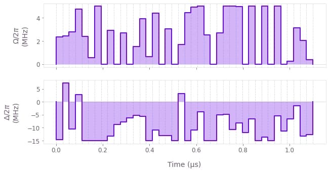
The above plots show the optimized pulses $\Omega (t)$ and $\Delta (t)$ that produce the final state.
The next cell sets up a function to plot the optimized population dynamics and the final state. This involves simulating the dynamics using the full Hamiltonian, including optimized control terms.
def plot_result(result):
    # Get physical parameters for the simulation.
    qubit_count = result["qubit_count"]
    omega_signal = result["omega"]
    delta_signal = result["delta"]
    krylov_subspace_dimension = result["krylov_subspace_dimension"]

    graph = bo.Graph()

    # Create initial and target states.
    initial_state = graph.fock_state(2**qubit_count, 0)
    target_state = create_target_state(qubit_count)

    # Calculate terms and put together the full Hamiltonian.
    H_omega, H_delta, H_fixed = get_rydberg_hamiltonian_terms(qubit_count)
    hamiltonian = graph.sparse_pwc_sum(
        [
            graph.sparse_pwc_operator(
                signal=graph.pwc(**omega_signal), operator=H_omega
            ),
            graph.sparse_pwc_operator(
                signal=graph.pwc(**delta_signal), operator=H_delta
            ),
            graph.constant_sparse_pwc_operator(duration=duration, operator=H_fixed),
        ]
    )

    sample_times = np.linspace(0, duration, 200)

    # Evolve the initial state.
    evolved_states = graph.state_evolution_pwc(
        initial_state=initial_state,
        hamiltonian=hamiltonian,
        krylov_subspace_dimension=krylov_subspace_dimension,
        sample_times=sample_times,
        name="evolved_states",
    )

    states = bo.execute_graph(graph, "evolved_states")

    # Data to plot.
    idx_even = sum(2**n for n in range(0, qubit_count, 2))
    idx_odd = sum(2**n for n in range(1, qubit_count, 2))
    densities_t = abs(np.squeeze(states["output"]["evolved_states"]["value"])) ** 2
    initial_density_t = densities_t[:, 0]
    final_density_t = densities_t[:, idx_odd] + densities_t[:, idx_even]
    target_density = np.abs(target_state) ** 2

    # Style and label definitions.
    bar_labels = [""] * 2**qubit_count
    bar_labels[idx_odd] = rf"$|{'10' * (qubit\_count // 2)}\rangle$"
    bar_labels[idx_even] = rf"$|{'01'* (qubit\_count // 2)}\rangle$"

    def bar_plot(ax, density, title):
        ax.bar(
            np.arange(2**qubit_count),
            density,
            edgecolor=qv.QCTRL_STYLE_COLORS[0],
            color=qv.QCTRL_STYLE_COLORS[0] + "4C",
            tick_label=bar_labels,
            linewidth=2,
        )
        ax.set_title(title)
        ax.set_ylabel("Population")

    gs = mpl.gridspec.GridSpec(2, 2, hspace=0.3)
    fig = plt.figure(figsize=(15, 10))
    fig.suptitle("Optimized state preparation", y=0.95)

    # Plot optimized final state and target state.
    ax = fig.add_subplot(gs[0, 0])
    bar_plot(ax, densities_t[-1], "Optimized final state")

    ax = fig.add_subplot(gs[0, 1])
    bar_plot(ax, target_density, "Target GHZ state")

    # Plot time evolution of basis state population.
    ax = fig.add_subplot(gs[1, :])
    ax.plot(sample_times / 1e-6, densities_t, "gray", linewidth=0.5)
    ax.plot(sample_times / 1e-6, initial_density_t, qv.QCTRL_STYLE_COLORS[1])
    ax.plot(sample_times / 1e-6, final_density_t, qv.QCTRL_STYLE_COLORS[0])
    ax.set_xlabel("Time (µs)")
    ax.set_ylabel("Population")
    ax.set_title("Basis states (gray), ground state (red), and target state (purple)")
plot_result(result)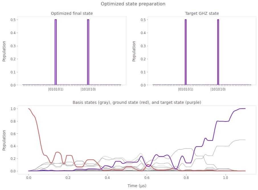
The plots show: (top) Final state obtained with the optimized pulses (left) and target state (right). These states are indistinguishable, with infidelity below $10^{-4}$. (bottom) Time evolution of the populations during the optimized pulse sequence, for all basis states (gray), the ground state (red), and the target state (purple). Note that since the target GHZ state is a superposition of two basis states, these two also show in gray as having a population of 0.5 at the end of the pulse.
Optimizing Boulder Opal pulses for up to 12 atoms
We proceed in the same way as in the previous section to optimize the GHZ generation for different numbers of atoms.
# Run optimization or load data.
use_saved_data = True

# List to store the results of all runs.
optimization_results = []

for n in [4, 6, 8, 10, 12]:
    # Run an optimization for various number of qubits.
    if use_saved_data:
        result = load_variable(f"./resources/Rydberg_{n}atoms_3optimizations.json")
        print("\n Optimization results with:")
        print(f"\t{result['qubit_count']} qubits")
        print(f"\t{result['segment_count']} segments")
        print(f"\t{result['optimization_count']} optimization count")
        print(f"Infidelity reached: {result['infidelity']:.1e}")
    else:
        result = optimize_GHZ_state(
            qubit_count=n, segment_count=40, optimization_count=3
        )
        save_variable(f"./resources/Rydberg_{n}atoms_3optimizations.json", result)

    # Store in the list to plot below
    optimization_results.append(result)
Optimization results with:
4 qubits
40 segments
3 optimization count
Infidelity reached: 8.4e-09
Optimization results with:
6 qubits
40 segments
3 optimization count
Infidelity reached: 8.3e-06
Optimization results with:
8 qubits
40 segments
3 optimization count
Infidelity reached: 1.0e-03
Optimization results with:
10 qubits
40 segments
3 optimization count
Infidelity reached: 2.7e-02
Optimization results with:
12 qubits
40 segments
3 optimization count
Infidelity reached: 7.6e-02
Plots of the final states and populations are similar to those for $N=6$ above, so here just the final state fidelities are displayed for different atom numbers.
# Get infidelity and number of qubits of each run.
infidelities = []
Nqs = []
for parameters in optimization_results:
    Nq, infid = parameters["qubit_count"], parameters["infidelity"]
    Nqs.append(Nq)
    infidelities.append(infid)
Nqs = np.array(Nqs)
infidelities = np.array(infidelities)

# Plot fidelities/infidelities vs number of qubits.
fig, axs = plt.subplots(1, 2, figsize=(15, 5))
fig.suptitle("Optimization performance", y=1)

ax = axs[0]
ax.plot(Nqs, 1 - infidelities, "o-")
ax.set_title("Fidelities")
ax.set_xlabel("Number of atoms")
ax.set_xticks([4, 6, 8, 10, 12])

ax = axs[1]
ax.semilogy(Nqs, infidelities, "o-")
ax.set_title("Infidelities (log scale)")
ax.set_xlabel("Number of atoms")
ax.set_xticks([4, 6, 8, 10, 12])
plt.show()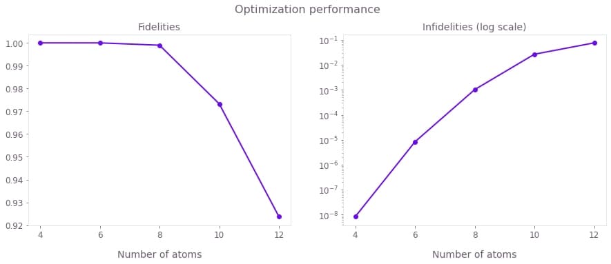
The above figures display the GHZ state generation fidelities (left) and infidelities (right) achieved for different numbers of atoms. Although it is generally harder to obtain better infidelities for larger atomic arrays, using Boulder Opal optimized pulses you can obtain fidelities of over 0.99.
Effects of spontaneous emission using the jump-based trajectory method
We now investigate the effect spontaneous emission from the Rydberg state has on the final state using the graph.jump_trajectory_evolution_pwc node, which is Boulder Opal's jump-based trajectory method.
Spontaneous emission caused by the decay of the Rydberg state is an incoherent process. In order to simulate this we use the Lindblad master equation \begin{equation} \partial_t \rho = -i [H(t), \rho] + \sum_{l,j} L^{(l)}_j \rho L^{(l)\dagger}_j - \frac{1}{2} \{L^{(l)\dagger}_jL^{(l)}_j, \rho \}, \end{equation} where $l$ is an index over the atoms and $L^{(l)}_j = \sqrt{b_{jr}\gamma_r}\vert j \rangle_l \langle r \vert$ is a decay operator between the Rydberg state and the state $\vert j \rangle \in \{ \vert 0 \rangle, \vert d \rangle \}$. $\gamma_r$ is the decay rate of the Rydberg state, $b_{jr}$ are branching ratios to the lower levels and $\vert d \rangle$ is a "dark" state that represents hyperfine levels not used. Here we take $b_{0r} = 1/8$ and $b_{dr} = 7/8$ and will look at two different values for the Rydberg decay time, $\tau_r = [150~{\rm \mu s}, 540~{\rm \mu s}]$, noting the inverse relationship between the decay time and the decay rate, $\gamma_r=1/\tau_r$
def simulate_with_decay(result, tau_r, run_async):
    # Get physical parameters for the simulation.
    qubit_count = result["qubit_count"]
    omega_signal = result["omega"]
    delta_signal = result["delta"]
    interaction_strength = result["interaction_strength"]
    graph = bo.Graph()

    # Create initial and target states.
    initial_state = graph.fock_state(3**qubit_count, 0)

    # Calculate terms and put together the full Hamiltonian.
    H_omega, H_delta, H_fixed = get_rydberg_hamiltonian_terms(
        qubit_count, level_count=3, interaction_strength=interaction_strength
    )
    hamiltonian = graph.sparse_pwc_sum(
        [
            graph.sparse_pwc_operator(
                signal=graph.pwc(**omega_signal), operator=H_omega
            ),
            graph.sparse_pwc_operator(
                signal=graph.pwc(**delta_signal), operator=H_delta
            ),
            graph.constant_sparse_pwc_operator(duration=duration, operator=H_fixed),
        ]
    )

    # Define single atom decay operators.
    decay_states = [0, 2]  # (0, d states)
    branching_ratios = [1 / 8, 7 / 8]
    Ls_single = []
    for decay_state, branching_ratio in zip(decay_states, branching_ratios):
        L = np.zeros((3, 3))
        L[decay_state, 1] = 1
        Ls_single.append((branching_ratio * (1 / tau_r), L))

    # Lindblad terms for all atoms
    Ls = [
        (gamma, graph.embed_operators([(L_single, atom)], [3] * qubit_count))
        for atom in range(qubit_count)
        for gamma, L_single in Ls_single
    ]

    # Perform jump-based trajectory evolution.
    evolved_states = graph.jump_trajectory_evolution_pwc(
        initial_state_vector=initial_state,
        hamiltonian=hamiltonian,
        lindblad_terms=Ls,
        max_time_step=duration * 1e-4,
        trajectory_count=100,
        name="evolved_density_matrices",
    )

    # Calculate infideltiy.
    target_state = create_target_state(6, level_count=3)
    target_matrix = np.outer(target_state, np.conj(target_state))
    infidelity = graph.density_matrix_infidelity(
        target_matrix, evolved_states, name="infidelity"
    )

    output_nodes = ["infidelity"]

    return bo.execute_graph(graph, output_nodes, run_async=run_async)
Here we will fix the number of qubits to $N=6$ and find optimal controls for different values of the interaction strength.
To demonstrate the effects of spontaneous emission, at each interaction strength, we calculate the evolved density matrix at the final time of the system Hamiltonian using graph.jump_trajectory_evolution_pwc.
The infidelity is measured by comparing the resulting density matrix with the target state.
The result of the optimization and the simulation with decay for varying interaction strengths and two different values for the decay rate is plotted below.
interactions = 2 * np.pi * 1e6 * np.array([2, 5, 10, 25, 50])
decay_times = [150e-6, 540e-6]
use_saved_data = True
if use_saved_data:
scan_results = load_variable("./resources/Rydberg_6atoms_decay_scans.json")
else:
scan_results = {}
scan_results["optimization_result"] = [
optimize_GHZ_state(optimization_count=3, interaction_strength=interaction)
for interaction in interactions
]
for decay in decay_times:
key = f"{int(1e6*decay)}"
scan_results[key] = {}
jobs = [
simulate_with_decay(result, tau_r=decay, run_async=True)
for result in scan_results["optimization_result"]
]
scan_results[key]["infidelities"] = [job.get_result() for job in jobs]
save_variable("./resources/Rydberg_6atoms_decay_scans.json", scan_results)fig, ax = plt.subplots(1, 1, figsize=(10, 5))
for key in scan_results.keys():
if key == "optimization_result":
infidelities = np.array([opt["result"]["cost"] for opt in scan_results[key]])
label = "Optimization performance"
else:
infidelities = [
result["output"]["infidelity"]["value"]
for result in scan_results[key]["infidelities"]
]
label = f"Simulation with decay time {key} $\mu$s"
ax.plot(interactions / (2 * np.pi * 1e6), infidelities, marker="o", label=label)
ax.set_xlabel("Interaction strength (MHz)")
ax.set_ylabel("Infidelity")
ax.set_yscale("log")
ax.set_xscale("log")
ax.legend(loc="best", bbox_to_anchor=(1, 1))
plt.suptitle("Final state infidelity (log scale)")
plt.show()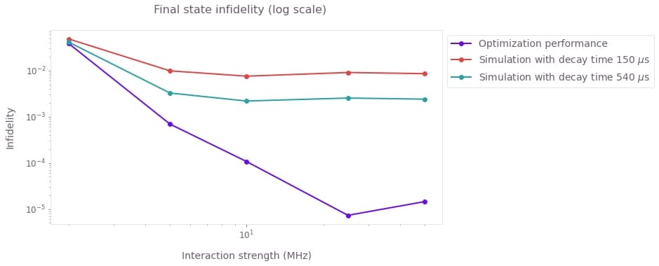
Here we see that by including the spontaneous emission into the simulation, the final state fidelity degrades by a few order of magnitudes. As expected, the effect is worse for shorter decay times.
