Design robust pulses for widefield microscopy with NV centers
Increasing detection area by $>10\times$ using $\pi$ pulses robust to field inhomogeneities across large diamond chips
Boulder Opal enables generation of controls robust to diverse noise sources in state-of-the-art quantum sensing applications. One of the prominent quantum sensor for room temperature and biocompatible applications is based on nitrogen-vacancy (NV) centers in diamond. In the their common widefield configuration, the NV sensors provide powerful microscopic 2D-imaging of magnetic and electric fields, as well as temperature emanating from the samples deposited on the sensor. In this configuration, NV centers are embedded near the surface of a relatively large diamond sensing chip leaving the sensor exposed to field inhomogeneities that limit the effective detection area.
In this application note we address this problem by designing $\pi$ pulses that are robust to microwave and background magnetic field inhomogeneities experienced by the NV centers. We demonstrate that such pulses can increase the effective sensing area by more than 10 times as compared to a simple square pulse in the case of a widefield diamond sensor subjected to strong inhomogeneities produced by a loop resonator.
Imports and basic setup
import jsonpickle
import numpy as np
import matplotlib.pyplot as plt
from matplotlib.colors import LinearSegmentedColormap, TwoSlopeNorm
from matplotlib.cm import ScalarMappable

import qctrlvisualizer as qv
import boulderopal as bo

plt.style.use(qv.get_qctrl_style())


# Read and write helper functions, type independent.
def save_variable(file_name, var):
    """
    Save a single variable to a file using jsonpickle.
    """
    with open(file_name, "w+") as file:
        file.write(jsonpickle.encode(var))


def load_variable(file_name):
    """
    Load a variable from a file encoded with jsonpickle.
    """
    with open(file_name, "r+") as file:
        return jsonpickle.decode(file.read())


colors = {"Q-CTRL": qv.QCTRL_STYLE_COLORS[0], "Square": qv.QCTRL_STYLE_COLORS[1]}
use_saved_data = True
Model of the NV center under inhomogeneous field noises
The ground state of a negatively charged NV center is described by the following Hamiltonian: \begin{equation} H = DS_z^2 + \gamma_e B_0 S_z + \gamma_e B_1(\cos(\omega t +\phi)S_x + \sin(\omega t +\phi)S_y), \end{equation} where $S_{x,y,z}$ are the $S=1$ spin operators and $\gamma_e$ is the gyromagnetic ratio of an electron. The $|\pm1\rangle$ levels are separated from $|0\rangle$ by the zero-field splitting $D=2.87$ GHz. The background magnetic field $B_0$ is applied along the direction of the NV center quantization axis. The driving field used to control the spin transitions has an amplitude $B_1(t)$, frequency $\omega$, and relative phase $\phi$.
We will run the pulses on one of two spin transitions using the resonant frequency $\omega=D-\gamma_eB_0$ for control of the $|0\rangle \leftrightarrow |-1\rangle$ transition. In the regime where $D+\gamma_eB_0\gg \gamma_eB_1$, we can effectively reduce the Hamiltonian to a two-level system \begin{align} H = D\frac{\sigma_z}{2} - \gamma_e B_0 \frac{\sigma_z}{2} + \gamma_e B_1(t)\left[\cos(\omega t +\phi)\frac{\sigma_x}{2} + \sin(\omega t +\phi)\frac{\sigma_y}{2}\right] , \end{align} where $\sigma_{x,y,z}$ are Pauli matrices. Finally, moving into the rotating frame, the Hamiltonian can be expressed as \begin{align} H = \Omega(t)\frac{\sigma_x}{2} , \end{align} where the driving field has been absorbed into the complex Rabi rate $\Omega(t)= \gamma_e B_1(t)e^{i\phi(t)}$. The Hamiltonian is subjected to noise in the following way: \begin{align} H = (1+\beta)\Omega(t)\frac{\sigma_x}{2} + \delta \frac{\sigma_z}{2}, \end{align} where the parameter $\beta$ represents the variations in the Rabi rate caused by microwave field inhomogeneities across the diamond, while the parameter $\delta$ represents detuning noise caused by inhomogeneities in the background magnetic field $B_0$ or by the hyperfine shifts due to local nuclear spin.
Generating robust pulses
In the cell below we show how to generate robust pulses using a stochastic optimizer.
For details on how to set up this kind of optimization please refer to this user guide.
In this example, the parameter $\beta$ will be sampled from a Gaussian distribution with standard deviation $\sigma_{\beta} = 0.4$ (sigma_beta), while $\delta$ is sampled from a Gaussian distribution with a standard deviation that covers the extent of the hyperfine splitting $\sigma_{\delta}=1.5$MHz (sigma_delta).
Note that the effects of hyperfine interaction can be refined by an easy expansion of the Hamiltonian to include the nitrogen spin. The noises are introduced as a batch of ($\beta$, $\delta$) quasi-static points of a specified size (noise_sample_count).
Noise in each quasi-static point leads to a distinct Hamiltonian, allowing the optimizer to find the pulse that is simultaneously valid across a wide range of system inhomogeneities.
omega_max = 2 * np.pi * 10e6  # Maximum Rabi rate.
duration = 400e-9  # s
segment_count = 300  # Number of pulse segments.

optimization_variable_count = 100  # Degrees of freedom for the optimizer.
cutoff_frequency = 6 * omega_max  # Pulse frequency bandwidth limit.
sigma_beta = 0.4
sigma_delta = 2 * np.pi * 1.5e6
noise_sample_count = 200  # Number of samples from the noise ditibutions.
iteration_count = 2000

pi_pulse_controls = {}

if use_saved_data:
    results = load_variable("./resources/NV_widefield_pi_pulse")
else:
    print("**Optimizing pulse**")
    graph = bo.Graph()

    # Define the unitary operation of the optimized pulse.
    target_operator = graph.pauli_matrix("X")

    # Set up for optimizable controls.
    unfiltered_drive_signal = graph.complex_optimizable_pwc_signal(
        segment_count=optimization_variable_count, duration=duration, maximum=omega_max
    )
    # Filter drive signal to incorporate band limits.
    filtered_signal = graph.filter_and_resample_pwc(
        pwc=unfiltered_drive_signal,
        kernel=graph.sinc_convolution_kenrel(cutoff_frequency),
        segment_count=segment_count,
    )

    # Add envelope to pin signal to zero at start/end.
    envelope = graph.signals.cosine_pulse_pwc(
        duration=duration,
        segment_count=segment_count,
        amplitude=1.0,
        flat_duration=0.9 * duration,
    )
    drive_signal = envelope * filtered_signal
    drive_signal.name = r"$\Omega$"

    # Generate noise points to build robustness.
    # Noise representing Rabi rate inhomogeneities.
    betas = graph.random.normal(
        mean=0, standard_deviation=sigma_beta, shape=(noise_sample_count,)
    )
    # Noise representing inhomogenties in B0 and line shifts due to hyperfine coupling.
    deltas = graph.random.normal(
        mean=0, standard_deviation=sigma_delta, shape=(noise_sample_count,)
    )

    # Construct Hamiltonian terms.
    # Set up drive term.
    drive_term = graph.hermitian_part(drive_signal * graph.pauli_matrix("M"))

    # Set up quasi-static noise point terms.
    beta_signal = graph.constant_pwc(
        constant=betas, duration=duration, batch_dimension_count=1
    )
    delta_signal = graph.constant_pwc(
        constant=deltas, duration=duration, batch_dimension_count=1
    )
    delta_term = delta_signal * graph.pauli_matrix("Z") / 2.0

    # Add noise points to Hamiltonian.
    quasistatic_hamiltonian = (1 + beta_signal) * drive_term + delta_term

    # Set up cost as sum of all infidelities.
    infidelities = graph.infidelity_pwc(
        hamiltonian=quasistatic_hamiltonian, target=graph.target(target_operator)
    )
    cost = graph.sum(infidelities, name="cost")

    # Run optimization.
    results = bo.run_stochastic_optimization(
        graph=graph,
        cost_node_name="cost",
        output_node_names=r"$\Omega$",
        iteration_count=iteration_count,
    )
    save_variable("./resources/NV_widefield_pi_pulse", results)

pi_pulse_controls["Q-CTRL"] = results["output"]

# Plot controls.
qv.plot_controls(pi_pulse_controls["Q-CTRL"], polar=False, smooth=True)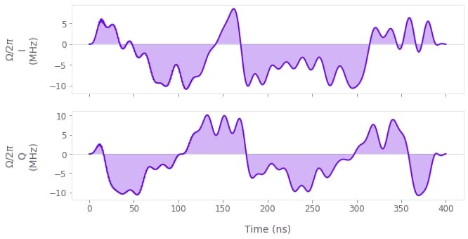
The plot above shows the I and Q components of the optimized $\pi$ pulse. Note that this pulse is relatively long because it individually has to fulfill all of the robustness constraints. However, if optimized in the context of a pulse sequence (outside the scope of this notebook), the constraints can be distributed across the entire sequence, thereby allowing the individual $\pi$ pulses to be shorter.
Robustness characterization
We will now verify the robustness of the pulse by comparing its performance with that of a simple square pulse with the same maximum Rabi rate, as defined below.
pi_pulse_controls["Square"] = {
    r"$\Omega$": {
        "durations": np.array([np.pi / omega_max]),
        "values": np.array([omega_max]),
    }
}
qv.plot_controls(pi_pulse_controls["Square"])
plt.show()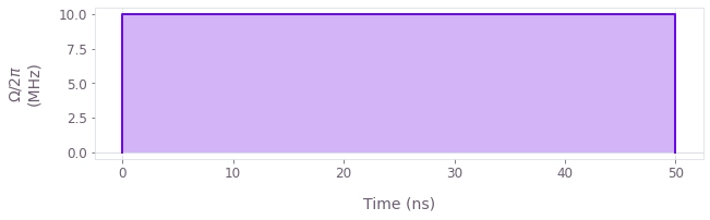
The cell below performs a quasi-static scan over the range of $\beta$ values, enabling us to plot the pulse infidelity as a function of noise amplitude and compare the robustness for the optimized and square pulses.
betas = np.linspace(-0.9, 0.9, 50)
scan_infidelities = {}

schemes = ["Square", "Q-CTRL"]
for scheme in schemes:
    # Construct a batch of pulses experiencing different driving strengths.
    scan_controls = pi_pulse_controls[scheme]
    durations = scan_controls[r"$\Omega$"]["durations"]
    values = scan_controls[r"$\Omega$"]["values"]
    omega_values = values * (1.0 + betas)[:, None]

    # Set up the graph for the quasi-static scan simulation.
    graph = bo.Graph()
    omega_signal = graph.pwc(values=omega_values, durations=durations, time_dimension=1)
    hamiltonian = graph.hermitian_part(omega_signal * graph.pauli_matrix("M"))

    # Infidelities for detuning rates.
    infidelities = graph.infidelity_pwc(
        hamiltonian=hamiltonian,
        target=graph.target(graph.pauli_matrix("X")),
        name="infidelities",
    )

    # Calculate the graph and extract infidelities.
    graph_result = bo.execute_graph(graph, "infidelities")

    scan_infidelities[scheme] = graph_result["output"]["infidelities"]["value"]
Your task (action_id="1827934") is queued.
Your task (action_id="1827934") has started.
Your task (action_id="1827934") has completed.
Your task (action_id="1827943") is queued.
Your task (action_id="1827943") has started.
Your task (action_id="1827943") has completed.
for scheme in ["Square", "Q-CTRL"]:
    plt.plot(betas, scan_infidelities[scheme], color=colors[scheme], label=scheme)
plt.xlabel(r"$\beta$")
plt.ylabel("Infidelity")
plt.suptitle("Quasi-static scan")
plt.legend()
plt.ylim([0, 1])
plt.xlim([-1, 1])
plt.show()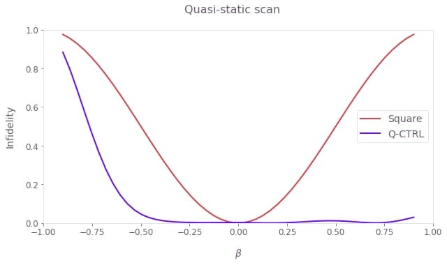
Observe that the square pulse loses its fidelity rapidly. In contrast, the optimized pulse achieves the targeted unitary operation successfully over a wide range of variations in the Rabi rate. Note that the optimized pulse remains robust to losses of the driving field amplitude up to half its peak value.
Simulating the pulse performance against spatial inhomogeneities
In this section we simulate the state evolution of NV sensors across the diamond chip surface subjected to strong microwave inhomogeneities such as those originating from a ring resonator, as shown in the figure below.
# Load data.
resonator_data = load_variable("./resources/NV_widefield_resonator_data")
rabi_profile = resonator_data["rabi_profile"]
x_points = resonator_data["x_points"]
y_points = resonator_data["y_points"]
X, Y = np.meshgrid(x_points, y_points)
plot_rabi_rates = rabi_profile * omega_max / (2 * np.pi * 1e6)

fig, ax = plt.subplots(figsize=(8, 5))
fig.suptitle("Rabi rate profile")
ax.set_xlabel("x (mm)")
ax.set_ylabel("y (mm)")
ax.set_aspect(1)

contours = plt.contour(
    X / 1e-3,
    Y / 1e-3,
    plot_rabi_rates,
    levels=np.array([0.9, 1.1]) * 10,
    colors="#6C5C71",
    linestyles="-",
    linewidths=0.75,
)
fmt = {level: label for level, label in zip(contours.levels, ["10%", "+10%"])}
plt.clabel(contours, inline=True, fmt=fmt, fontsize=10)

qctrl_cmap = LinearSegmentedColormap.from_list(
    "Q-CTRL_colormap",
    ["#C02C21", "#FA7370", "#FED6D7", "#FFFFFF", "#EDE0FE", "#B482FA", "#680CE9"],
    N=200,
)
extent = 1e3 * np.array([min(x_points), max(x_points), min(y_points), max(y_points)])
image = plt.contourf(
    plot_rabi_rates,
    extent=extent,
    levels=100,
    cmap=qctrl_cmap,
    norm=TwoSlopeNorm(vcenter=10.0),
)
cbar = fig.colorbar(image, ticks=np.arange(2, 17, 2))
cbar.set_label(label="Rabi rate (MHz)")

plt.show()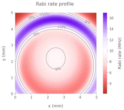
The profile above shows the Rabi rate inhomogeneities with spatial variations across the widefield sensor area that will be used in the simulation. The chip is assumed to be uniformly populated by the NV centers while effects of coherence time limits are omitted for clarity. The pulse durations are set by the ideal Rabi rate (white in the image above), causing the variations to impact the effective signal contrast by limiting the maximal population inversion achieved by the $\pi$ pulses.
states_pi_pulse = {}
for scheme, controls in pi_pulse_controls.items():
    durations = controls[r"$\Omega$"]["durations"]
    phasors = controls[r"$\Omega$"]["values"]

    # Construct a 2D profile of Rabi rate inhomogeneities in a batch format.
    phasors = phasors * rabi_profile[:, :, None]

    duration = np.sum(durations)
    initial_state = np.array([1.0, 0.0])

    # Start graph definition.
    graph = bo.Graph()
    omega_signal = graph.pwc(values=phasors, durations=durations, time_dimension=-1)
    hamiltonian = graph.hermitian_part(omega_signal * graph.pauli_matrix("M"))

    # Infidelities for detuning rates.
    unitaries = graph.time_evolution_operators_pwc(
        hamiltonian=hamiltonian, sample_times=[duration], name="unitaries"
    )
    evolved_states = unitaries @ initial_state[:, None]
    evolved_states.name = "evolved_states"

    # Execute the graph.
    result = bo.execute_graph(graph, ["evolved_states", "unitaries"])
    # Extract and return infidelities.
    states_pi_pulse[scheme] = result["output"]["evolved_states"]["value"][:, :, 0, :, 0]
Your task (action_id="1827965") is queued.
Your task (action_id="1827965") has started.
Your task (action_id="1827965") has completed.
Your task (action_id="1827972") is queued.
Your task (action_id="1827972") has started.
Your task (action_id="1827972") has completed.
We now compare the widefield performance of the sensor under the square and the optimized pulses.
fig, axs = plt.subplots(1, 3, figsize=(18, 5))

contour_area = {}
for idx, (scheme, states) in enumerate(states_pi_pulse.items()):
    plot_state = 1
    populations = np.abs(states[:, :, plot_state]) ** 2
    contour_area[scheme] = np.sum(populations > 0.99)

    axs[idx].set_title(f"{scheme} π pulse")
    axs[idx].set_xlabel("x (mm)")
    axs[idx].set_ylabel("y (mm)")
    axs[idx].set_aspect(1)

    # Contours.
    contours = axs[idx].contour(
        X / 1e-3,
        Y / 1e-3,
        populations,
        levels=[0.7, 0.99],
        colors=["#6C5C71", "#E9E7EA"],
        linewidths=0.75,
    )
    axs[idx].clabel(contours, inline=True, fontsize=10)
    # Gradient image.
    image = axs[idx].contourf(
        populations,
        extent=extent,
        levels=300,
        cmap=qctrl_cmap,
        norm=TwoSlopeNorm(vcenter=0.9, vmin=0.0, vmax=1.0),
    )
cbar = fig.colorbar(
    ScalarMappable(cmap=qctrl_cmap),
    ticks=np.arange(0.0, 2, 0.2),
    ax=[axs[0], axs[1]],
    pad=0.03,
    shrink=0.92,
)
cbar.set_label(r"$P\_{|-1\rangle}$")

# Bar chart.
boost = contour_area["Q-CTRL"] / contour_area["Square"]

axs[2].set_title(f"{boost:1.1f}× sensing area boost")
axs[2].set_ylabel("Relative surface area, >99% fidelity", labelpad=10)
axs[2].set_xlim(0, 2)
x_pos = [0.5, 1.5]
axs[2].set_xticks(x_pos, colors.keys())
axs[2].bar(x_pos, [boost, 1], width=0.4, color=colors.values())

plt.show()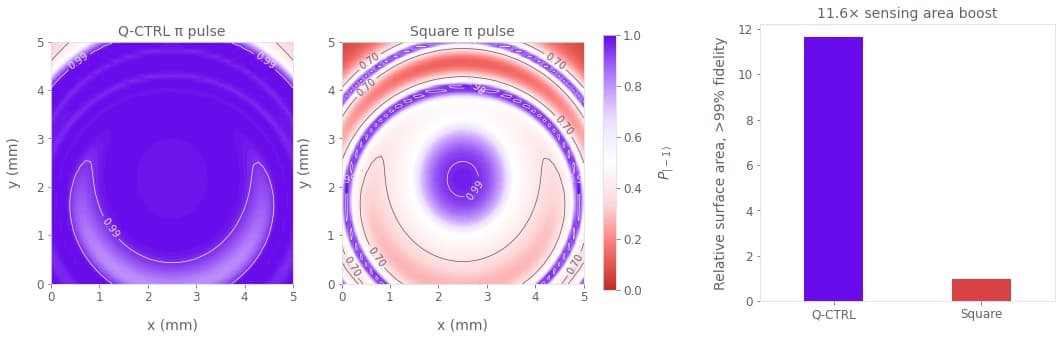
We see the population contrast achieved by the pulses over the entire field of view of the chip. The performance of the square pulse diminishes quickly with the Rabi rate deviation, leaving only a small area of high effective contrast. In comparison, the optimized pulse achieves uniform performance over most of the sensing area.
Overall we see that in this particular example, the optimized pulse expands the area of 99% effective contrast by over 10 times. However, it's worth noting that our optimization strategy generates pulses whose performance does not depend on the specific manifestation of the spatial inhomogeneities, making the optimized pulses versatile in NV sensing applications under varying environmental conditions.