Design error-detectable entangling gates for superconducting resonators in dual-rail encoding
Robust $ZZ_\Theta$ gate with a transmon ancilla engineered using Boulder Opal
Boulder Opal is a versatile tool for the numerical optimization of controls in quantum systems. It provides a flexible optimization engine that can be applied to both unitary operations and individual states and, furthermore, allows for the straightforward incorporation of arbitrary additional objectives such as the robustness of the pulses. With Boulder Opal, nonlinearities and complex interactions of the various system components can be easily accounted for, which not only introduce coherent errors, but also open up new possibilities for the error-robust processing of quantum information.
Tsunoda et al. have proposed a scheme to implement entangling gates on bosonically encoded qubits using a transmon ancilla that makes first-order errors detectable. On the path towards fault-tolerant quantum computation, dual-rail qubits are particularly promising as they leverage the intrinsic noise bias of superconducting cavities to allow for a favorable error hierarchy while requiring only a single excitation per logical qubit. A logical dual-rail qubit is encoded by a photon in one of two cavity modes, $|0\rangle_L = |01\rangle$, $|1\rangle_L = |10\rangle$.
In this application note, we demonstrate how Boulder Opal can be used to design an optimal robust pulse sequence to execute an error-detectable $ZZ_\Theta$ gate on superconducting resonators in dual-rail encoding. We will cover:
- Performing model-based control optimizations for the individual gates constituting the logical $ZZ_\Theta$ gate.
- Adding robustness against pulse shaping errors as an objective in the optimizations.
- Validating the performance of the pulse sequences in an open system.
Imports and initialization
import jsonpickle
import numpy as np

import matplotlib.pyplot as plt
from matplotlib.colors import LogNorm
import qctrlvisualizer as qv

import boulderopal as bo

bo.cloud.set_verbosity("QUIET")

plt.style.use(qv.get_qctrl_style())
Gate construction in the dual-rail cavity system with a transmon ancilla
While two dual-rail encoded qubits require, in principle, four physical cavity modes, it suffices to facilitate an interaction between two of them to realize a two-qubit gate. Thus, the system we consider consists of two superconducting cavities $A$ and $B$, one of which couples dispersively to a transmon ancilla. In a suitable frame, the system can be modeled by the Hamiltonian \begin{align} H &= H_\text{BS} + H_{\chi} + H_\text{NL}, \\ H_\text{BS}/\hbar &= g(t) a^\dagger b + g^*(t) ab^\dagger + \Delta_\text{BS}(t) a^\dagger a, \\ H_{\chi}/\hbar &= -\frac{\chi}{2}\sigma_z a^\dagger a + \epsilon(t) |g\rangle \langle f| + \epsilon^*(t) |f\rangle \langle g | + \Delta_\epsilon |f\rangle \langle f|, \\ H_\text{NL}/\hbar &= -\frac{K_a}{2}a^\dagger a^\dagger a a - \frac{K_b}{2} b^\dagger b^\dagger b b + a^\dagger a^\dagger a a (\chi_f'|f\rangle \langle f| + \chi_e' |e\rangle \langle e|) + \chi_{ab}a^\dagger a b^\dagger b. \end{align}
The Hamiltonian $H_\text{BS}$ describes the effective beamsplitter interaction between the two bosonic modes $A$ and $B$ with annihilation operators $a$ and $b$, respectively. This interaction can be engineered via the complex drive strength $g(t)$ and the effective detuning $\Delta_\text{BS}(t)$. One of the cavities, here cavity $A$, interacts dispersively at rate $\chi$ with the transmon ancilla as described by $H_\chi$. Note that we concentrate on the $\{|g\rangle,|f\rangle \}$ transmon subspace so that $\sigma_z = |g\rangle \langle g| - |f\rangle \langle f|$, while making use of the $|e\rangle$ level to detect ancilla decay when working in the open system. We assume that the $|g\rangle \leftrightarrow |f\rangle$ transition can be directly addressed with a pulse at Rabi rate $\epsilon(t)$ which is detuned from resonance by $\Delta_\epsilon$. The Hamiltonian $H_\text{NL}$ models higher-order corrections, including the self-Kerr of the individual cavities at rate $K_a$ and $K_b$, the corrections to the dispersive interaction, $\chi_f'$ and $\chi_e'$, as well as the cross-Kerr of the two cavity modes at rate $\chi_{ab}$.
To construct an error-detectable $ZZ_\Theta$ gate on two qubits in dual-rail encoding, Tsunoda et al. proposed the following gate sequence
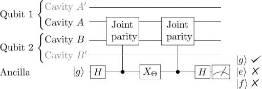
which enables the detection of first-order errors when not measuring the ancilla in the ground state at the end of the protocol. This is of interest for near-term protocols relying on postselection as well as for an embedding into error correction codes. Parametrization of the logical two-qubit gate can be easily implemented via the corresponding ancilla rotation. Together with single-qubit rotations mediated by a beamsplitter interaction between the two cavities belonging to the same logical qubit, the $ZZ_\Theta$ gate forms a universal gate set.
Designing optimal control pulses for the individual gates
To find optimal pulses realizing the error-detectable $ZZ_\Theta$ gate on the dual-rail qubits, we perform individual optimizations for the gates in the sequence.
We start by defining all relevant parameters, states, and operators. As an example, in the following, we focus on the case $\Theta=\pi/2$.
# Gate parameters.
theta = np.pi / 2  # Gate angle
gate_duration_h = 100e-9  # s # Duration of the Hadamard gate.
gate_duration_c_parity = 500e-9  # s # Duration of the controlled joint parity gate.
gate_duration_rx = 40e-9  # s # Duration of the RX gate.
gate_duration_tot = 2 * gate_duration_h + 2 * gate_duration_c_parity + gate_duration_rx

# System and coupling parameters.
chi = (
    -2 * np.pi * 2e6
)  # rad.Hz # dispersive coupling between cavity A and transmon ancilla
k_a = 2 * np.pi * 2e3  # rad.Hz # self-Kerr of cavity A
k_b = 2 * np.pi * 2e3  # rad.Hz # self-Kerr of cavity B
chi_f_prime = 2 * np.pi * 2e3  # rad.Hz
chi_e_prime = 2 * np.pi * 1.125e3  # rad.Hz
chi_ab = 2 * np.pi * 100  # rad.Hz

# Simulation and optimization parameters.
cavity_dim = 3  # Cavity dimension.
transmon_dim = 3  # Transmon dimension.
max_rabi_rate_c = 2 * np.pi * 5e6  # rad.Hz # Maximum cavity drive.
max_rabi_rate_t = 2 * np.pi * 30e6  # rad.Hz # Maximum transmon drive.
optimizer_variable_count = 64
segment_count = 128
sinc_cutoff_frequency_drives = 2 * np.pi * 4e7  # rad.Hz

# Error ranges for robust optimization.
sample_count_optimization = 5
amplitude_errors_optimization = np.linspace(
    -0.025, 0.025, num=sample_count_optimization
)

# Gate we ultimately want to implement.
rzz = np.diag(np.exp(1j * theta / 2 * np.array([-1, 1, 0, 1, -1, 0, 0, 0, 0])))
rzz_tot = np.kron(rzz, np.eye(transmon_dim))

# Hadamard gate on the transmon ancilla.
h = np.array([[1, 0, 1], [0, 0, 0], [1, 0, -1]]) / np.sqrt(2)
h_tot = np.kron(np.eye(cavity_dim), np.kron(np.eye(cavity_dim), h))

# Ancilla-controlled joint parity operation on the cavities.
c_parity = np.eye(cavity_dim * cavity_dim * transmon_dim)
c_parity[5, 5], c_parity[11, 11], c_parity[17, 17], c_parity[23, 23] = -1, -1, -1, -1

# RX gate on the transmon ancilla.
rx = np.array(
    [
        [np.cos(theta / 2), 0, -1j * np.sin(theta / 2)],
        [0, 0, 0],
        [-1j * np.sin(theta / 2), 0, np.cos(theta / 2)],
    ]
)
rx_tot = np.kron(np.eye(cavity_dim), np.kron(np.eye(cavity_dim), rx))

# Cardinal cavity states.
cardinal_states_c = [
    np.array([1, 0, 0]),
    np.array([0, 1, 0]),
    np.array([1, 1, 0]) / np.sqrt(2),
    np.array([1, -1, 0]) / np.sqrt(2),
    np.array([1, 1j, 0]) / np.sqrt(2),
    np.array([1, -1j, 0]) / np.sqrt(2),
]

# Pauli matrices for the transmon.
pauli_matrices = [
    np.array([[0, 0, 1], [0, 0, 0], [1, 0, 0]]),
    np.array([[0, 0, -1j], [0, 0, 0], [1j, 0, 0]]),
    np.array([[1, 0, 0], [0, 0, 0], [0, 0, -1]]),
]


def create_system_operators(graph, dim_c, dim_t):
    """
    Create the required system operators for the two cavities
    (of dimension dim_c) and the transmon ancilla (of dimension dim_t).
    """
    a = graph.embed_operators(
        (graph.annihilation_operator(dim_c), 0), [dim_c, dim_c, dim_t]
    )
    n_a = graph.adjoint(a) @ a
    b = graph.embed_operators(
        (graph.annihilation_operator(dim_c), 1), [dim_c, dim_c, dim_t]
    )
    n_b = graph.adjoint(b) @ b
    t = graph.embed_operators(
        (np.array([[0, 0, 1], [0, 0, 0], [0, 0, 0]]), 2), [dim_c, dim_c, dim_t]
    )
    n_t = graph.adjoint(t) @ t
    t_z = graph.embed_operators((np.diag([1, 0, -1]), 2), [dim_c, dim_c, dim_t])

    # Operators including transmon level e.
    t_e = graph.embed_operators(
        (graph.annihilation_operator(dim_t), 2), [dim_c, dim_c, dim_t]
    )
    n_t_e = graph.adjoint(t_e) @ t_e

    return (a, n_a, b, n_b, t, n_t, t_z, t_e, n_t_e)
For the optimization, we start with the gates that are independent of the specific rotation angle $\Theta$ as these gates can be reused for the optimization of the parametrized $ZZ_\Theta$ gate for arbitrary angles.
As a first step, we optimize the transmon pulses that implement the Hadamard gates. In addition to the infidelity of the realized and the target operation, we penalize deviations from the "equal-latitude condition". Adhering to this condition, which corresponds to the latitude of the transmon state in the $\{|g\rangle,|f\rangle \}$ subspace being independent of the cavity states, enables the detection of transmon dephasing errors occurring during the gate, see Tsunoda et al.. The weights of the terms in the cost function are determined empirically. To be able to take the different initial and final transmon latitudes for the two Hadamard gates in the sequence into account, the two gates are optimized individually.
def optimize_hadamard(initial_state_t, robust=False):
    graph = bo.Graph()

    # Optimizable transmon drive.
    drive_t = graph.complex_optimizable_pwc_signal(
        segment_count=optimizer_variable_count,
        duration=gate_duration_h,
        maximum=max_rabi_rate_t,
    )
    drive_t = graph.filter_and_resample_pwc(
        pwc=drive_t,
        kernel=graph.sinc_convolution_kernel(sinc_cutoff_frequency_drives),
        segment_count=segment_count,
        duration=gate_duration_h,
    )
    drive_t = drive_t * graph.signals.cosine_pulse_pwc(
        duration=gate_duration_h,
        segment_count=segment_count,
        amplitude=1.0,
        flat_duration=gate_duration_h - 10e-9,
    )
    drive_t.name = "drive_t"

    # Optimizable detuning for the transmon.
    delta_t = graph.optimizable_scalar(
        lower_bound=2 * chi, upper_bound=-2 * chi, name="delta_t"
    )

    # Setup of the Hamiltonian.
    _, n_a, _, n_b, t, n_t, t_z, _, n_t_e = create_system_operators(
        graph, cavity_dim, transmon_dim
    )
    h_drift = (
        -chi / 2 * n_a @ t_z
        - k_a / 2 * (n_a @ n_a - n_a)
        - k_b / 2 * (n_b @ n_b - n_b)
        + chi_f_prime * (n_a @ n_a - n_a) @ n_t
        + chi_e_prime * (n_a @ n_a - n_a) @ (n_t_e - 2 * n_t)
        + chi_ab * n_a @ n_b
    )
    h_drive = graph.hermitian_part(drive_t * graph.adjoint(t)) + delta_t * n_t
    hamiltonian = h_drift + h_drive

    # Infidelity of the target unitary operation and the operation we implement.
    target = graph.target(h_tot)
    if robust:
        noise_operators = [graph.hermitian_part(drive_t * graph.adjoint(t))]
    else:
        noise_operators = None
    infidelity = graph.infidelity_pwc(
        hamiltonian, target, noise_operators=noise_operators, name="infidelity"
    )

    # Construction of the latitude cost:
    # Transmon states during the gate.
    initial_states = graph.reshape(
        graph.kronecker_product_list(
            [
                np.array(cardinal_states_c)[:, None, :, None],
                np.array(cardinal_states_c)[None, :, :, None],
                initial_state_t[:, None],
            ]
        ),
        (len(cardinal_states_c) ** 2, 1, -1, 1),
    )

    sample_times = np.linspace(0, gate_duration_h, segment_count)
    unitaries = graph.time_evolution_operators_pwc(
        hamiltonian=hamiltonian, sample_times=sample_times
    )[None]
    evolved_states = (unitaries @ initial_states)[..., 0]
    states_t = graph.partial_trace(
        density_matrix=graph.outer_product(evolved_states, evolved_states),
        subsystem_dimensions=[cavity_dim, cavity_dim, transmon_dim],
        traced_subsystems=[0, 1],
    )

    # Transmon latitude and deviation for different initial cavity states.
    v = graph.real(
        graph.density_matrix_expectation_value(
            density_matrix=states_t, operator=np.array(pauli_matrices)[:, None, None]
        )
    )
    latitude = graph.arccos(v[2] / graph.sqrt(graph.sum(v**2, axis=0)), name="latitude")
    latitude_cost = graph.sum(
        [
            graph.abs(latitude[i + 1] - latitude[i])
            for i in range(len(cardinal_states_c) ** 2 - 1)
        ]
    )

    cost = infidelity + 1e-5 * latitude_cost
    cost.name = "cost"

    return bo.run_optimization(
        graph=graph,
        cost_node_name="cost",
        output_node_names=["drive_t", "delta_t", "infidelity"],
        optimization_count=10,
    )


initial_state_t_h_1 = np.array([1, 0, 0])
initial_state_t_h_2 = np.array([1, 0, 1]) / np.sqrt(2)

with bo.cloud.group_requests():
    # First Hadamard gate.
    result_h_1 = optimize_hadamard(initial_state_t_h_1)
    # Second Hadamard gate.
    result_h_2 = optimize_hadamard(initial_state_t_h_2)

print("Optimized first Hadamard gate.")
print(f"Cost: {result_h_1['cost']:.3e}")
print(f"Gate infidelity: {result_h_1['output']['infidelity']['value']:.3e}\n")

print("Optimized second Hadamard gate.")
print(f"Cost: {result_h_2['cost']:.3e}")
print(f"Gate infidelity: {result_h_2['output']['infidelity']['value']:.3e}")
Optimized first Hadamard gate.
Cost: 1.114e-05
Gate infidelity: 2.818e-06
Optimized second Hadamard gate.
Cost: 2.013e-05
Gate infidelity: 8.535e-06
After finding high-fidelity pulses for the Hadamard gates, in the next step, we optimize the ancilla-controlled joint parity gate that applies the operation $P = e^{i\pi\left(a^\dagger a + b^\dagger b \right)}$ to the cavity modes if the transmon is in state $|f\rangle$. The success of the gate is quantified for the cardinal cavity states lying on the axes of the logical Bloch sphere, for which we evaluate the average infidelity of the evolved states and the corresponding target states. Furthermore, the cost function includes the deviation of the transmon latitude from the equator over the gate duration. Note that the effective beamsplitter detuning can in principle vary with time. For the given setting and the desired gate, however, this does not affect the gate fidelity significantly, so we focus on a constant value $\Delta_{BS}(t) = \Delta_{BS}$.
def optimize_c_parity(robust=False):
    graph = bo.Graph()

    # Optimizable cavity drive for the beamsplitter interaction.
    drive_c = graph.complex_optimizable_pwc_signal(
        segment_count=2 * optimizer_variable_count,
        duration=gate_duration_c_parity,
        maximum=max_rabi_rate_c,
        initial_values=np.sqrt(3) / 2 * chi * np.ones(2 * optimizer_variable_count),
    )
    drive_c = graph.filter_and_resample_pwc(
        pwc=drive_c,
        kernel=graph.sinc_convolution_kernel(sinc_cutoff_frequency_drives),
        segment_count=2 * segment_count,
        duration=gate_duration_c_parity,
    )
    drive_c = drive_c * graph.signals.cosine_pulse_pwc(
        duration=gate_duration_c_parity,
        segment_count=2 * segment_count,
        amplitude=1.0,
        flat_duration=gate_duration_c_parity - 10e-9,
    )
    drive_c.name = "drive_c"

    # Optimizable detuning for the beamsplitter interaction.
    delta_c = graph.optimizable_scalar(
        lower_bound=2 * chi,
        upper_bound=-2 * chi,
        initial_values=2 * np.pi * 1e6,
        name="delta_c",
    )

    # Setup of the Hamiltonian.
    a, n_a, b, n_b, _, n_t, t_z, _, n_t_e = create_system_operators(
        graph, cavity_dim, transmon_dim
    )
    h_drift = (
        -chi / 2 * n_a @ t_z
        - k_a / 2 * (n_a @ n_a - n_a)
        - k_b / 2 * (n_b @ n_b - n_b)
        + chi_f_prime * (n_a @ n_a - n_a) @ n_t
        + chi_e_prime * (n_a @ n_a - n_a) @ (n_t_e - 2 * n_t)
        + chi_ab * n_a @ n_b
    )

    if robust:
        amplitude_error_pwc = graph.constant_pwc(
            amplitude_errors_optimization,
            duration=gate_duration_c_parity,
            batch_dimension_count=1,
        )
        h_drive = (1 + amplitude_error_pwc) * graph.hermitian_part(
            drive_c * graph.adjoint(a) @ b
        ) + delta_c * n_a
    else:
        h_drive = graph.hermitian_part(drive_c * graph.adjoint(a) @ b) + delta_c * n_a
    hamiltonian = h_drift + h_drive

    # Initial and target states.
    initial_state_t = np.array([1, 0, 1]) / np.sqrt(2)
    initial_states = graph.reshape(
        graph.kronecker_product_list(
            [
                np.array(cardinal_states_c)[:, None, :, None],
                np.array(cardinal_states_c)[None, :, :, None],
                initial_state_t[:, None],
            ]
        ),
        (len(cardinal_states_c) ** 2, 1, 1, -1, 1),
    )
    target_states = (c_parity @ initial_states)[..., 0, :, 0]

    # Time evolution.
    sample_times = np.linspace(0, gate_duration_c_parity, 2 * segment_count)
    unitaries = graph.time_evolution_operators_pwc(
        hamiltonian=hamiltonian, sample_times=sample_times
    )[None]
    evolved_states = unitaries @ initial_states

    # Infidelity of the target states and the evolved states.
    infidelity = graph.sum(
        graph.state_infidelity(evolved_states[..., -1, :, 0], target_states)
    ) / (len(cardinal_states_c) ** 2)
    if robust:
        infidelity /= sample_count_optimization
    infidelity.name = "infidelity"

    # Construction of the latitude cost:
    # Transmon states during the gate.
    if robust:
        no_error_idx = int((sample_count_optimization - 1) / 2)
    else:
        no_error_idx = 0
    evolved_states = evolved_states[:, no_error_idx, :, :, 0]

    states_t = graph.partial_trace(
        density_matrix=graph.outer_product(evolved_states, evolved_states),
        subsystem_dimensions=[cavity_dim, cavity_dim, transmon_dim],
        traced_subsystems=[0, 1],
    )

    # Transmon latitude and deviation from equator for different initial cavity states.
    v = graph.real(
        graph.density_matrix_expectation_value(
            density_matrix=states_t, operator=np.array(pauli_matrices)[:, None, None]
        )
    )
    latitude = graph.arccos(v[2] / graph.sqrt(graph.sum(v**2, axis=0)), name="latitude")
    latitude_cost = graph.sum(graph.abs(latitude - np.pi / 2)) / (
        len(cardinal_states_c) ** 2
    )

    cost = infidelity + 1e-2 * latitude_cost
    cost.name = "cost"

    return bo.run_optimization(
        graph=graph,
        cost_node_name="cost",
        output_node_names=["drive_c", "delta_c", "infidelity"],
        optimization_count=1,
    )


result_c_parity = optimize_c_parity()
print("Optimized ancilla-controlled joint parity gate.")
print(f"Cost: {result_c_parity['cost']:.3e}")
print(f"Gate infidelity: {result_c_parity['output']['infidelity']['value']:.3e}")
Optimized ancilla-controlled joint parity gate.
Cost: 1.494e-06
Gate infidelity: 1.382e-06
Having optimized the pulses for the fixed gates in the sequence, we turn to the parametrized transmon rotation. In our example of a logical $ZZ_{\pi/2}$ gate, we have to optimize the transmon drive to realize an $X_{\pi/2}$ gate. For the cost function, we evaluate the infidelity of the full gate sequence as well as the deviation of the transmon latitude from the equator during the $X_{\pi/2}$ gate.
def optimize_rx(result_h_1, result_h_2, result_c_parity, robust=False):
    graph = bo.Graph()

    # Optimizable transmon drive.
    drive_t = graph.complex_optimizable_pwc_signal(
        segment_count=optimizer_variable_count,
        duration=gate_duration_rx,
        maximum=max_rabi_rate_t,
    )
    drive_t = graph.filter_and_resample_pwc(
        pwc=drive_t,
        kernel=graph.sinc_convolution_kernel(sinc_cutoff_frequency_drives),
        segment_count=segment_count,
        duration=gate_duration_rx,
    )
    drive_t = drive_t * graph.signals.cosine_pulse_pwc(
        duration=gate_duration_rx,
        segment_count=segment_count,
        amplitude=1.0,
        flat_duration=gate_duration_rx - 10e-9,
    )
    drive_t.name = "drive_t"

    # Optimizable detuning for the transmon.
    delta_t = graph.optimizable_scalar(
        lower_bound=-max_rabi_rate_t / 2,
        upper_bound=max_rabi_rate_t / 2,
        name="delta_t",
    )

    # Setup of the Hamiltonian.
    a, n_a, b, n_b, t, n_t, t_z, _, n_t_e = create_system_operators(
        graph, cavity_dim, transmon_dim
    )
    h_drift = (
        -chi / 2 * n_a @ t_z
        - k_a / 2 * (n_a @ n_a - n_a)
        - k_b / 2 * (n_b @ n_b - n_b)
        + chi_f_prime * (n_a @ n_a - n_a) @ n_t
        + chi_e_prime * (n_a @ n_a - n_a) @ (n_t_e - 2 * n_t)
        + chi_ab * n_a @ n_b
    )
    h_drive = graph.hermitian_part(drive_t * graph.adjoint(t)) + delta_t * n_t
    hamiltonian_rx = h_drift + h_drive

    # Infidelity of the target unitary operation and the operation we implement.
    target = graph.target(rx_tot)
    infidelity_rx = graph.infidelity_pwc(hamiltonian_rx, target, name="infidelity_rx")

    # Construction of the latitude cost:
    # Calculation of the transmon states during the RX gate.
    initial_state_t_rx = np.array([1, 0, 1]) / np.sqrt(2)
    initial_states_rx = graph.reshape(
        graph.kronecker_product_list(
            [
                np.array(cardinal_states_c)[:, None, :, None],
                np.array(cardinal_states_c)[None, :, :, None],
                initial_state_t_rx[:, None],
            ]
        ),
        (len(cardinal_states_c) ** 2, 1, -1, 1),
    )
    initial_states_rx = c_parity @ initial_states_rx
    sample_times_rx = np.linspace(0, gate_duration_rx, segment_count)
    unitaries_rx = graph.time_evolution_operators_pwc(
        hamiltonian=hamiltonian_rx, sample_times=sample_times_rx
    )[None]
    evolved_states_rx = (unitaries_rx @ initial_states_rx)[..., 0]
    states_t_rx = graph.partial_trace(
        density_matrix=graph.outer_product(evolved_states_rx, evolved_states_rx),
        subsystem_dimensions=[cavity_dim, cavity_dim, transmon_dim],
        traced_subsystems=[0, 1],
    )

    # Transmon latitude and deviation from equator for different initial cavity states.
    v = graph.real(
        graph.density_matrix_expectation_value(
            density_matrix=states_t_rx, operator=np.array(pauli_matrices)[:, None, None]
        )
    )
    latitude_rx = graph.arccos(
        v[2] / graph.sqrt(graph.sum(v**2, axis=0)), name="latitude_rx"
    )

    # To avoid the singularity occurring in case of a maximally mixed state, the normalization of the transmon state is omitted if necessary.
    latitude_rx_vz = graph.arccos(v[2], name="latitude_rx_vz")
    latitude_cost = graph.sum(graph.abs(latitude_rx_vz - np.pi / 2)) / (
        len(cardinal_states_c) ** 2
    )
    latitude_cost.name = "latitude_cost"

    # Combining the pulses for the full gate sequence.
    pulse_list_c = [
        graph.constant_pwc(0, gate_duration_h),
        graph.pwc(**result_c_parity["output"]["drive_c"]),
        graph.constant_pwc(0, gate_duration_rx),
        graph.pwc(**result_c_parity["output"]["drive_c"]),
        graph.constant_pwc(0, gate_duration_h),
    ]
    pulse_list_delta_c = [
        graph.constant_pwc(0, gate_duration_h),
        graph.constant_pwc(
            result_c_parity["output"]["delta_c"]["value"], gate_duration_c_parity
        ),
        graph.constant_pwc(0, gate_duration_rx),
        graph.constant_pwc(
            result_c_parity["output"]["delta_c"]["value"], gate_duration_c_parity
        ),
        graph.constant_pwc(0, gate_duration_h),
    ]
    pulse_list_t = [
        graph.pwc(**result_h_1["output"]["drive_t"]),
        graph.constant_pwc(0, gate_duration_c_parity),
        drive_t,
        graph.constant_pwc(0, gate_duration_c_parity),
        graph.pwc(**result_h_2["output"]["drive_t"]),
    ]
    pulse_list_delta_t = [
        graph.constant_pwc(result_h_1["output"]["delta_t"]["value"], gate_duration_h),
        graph.constant_pwc(0, gate_duration_c_parity),
        graph.constant_pwc(delta_t, gate_duration_rx),
        graph.constant_pwc(0, gate_duration_c_parity),
        graph.constant_pwc(result_h_2["output"]["delta_t"]["value"], gate_duration_h),
    ]
    drive_c_seq = graph.time_concatenate_pwc(pulse_list_c, name="drive_c_seq")
    delta_c_seq = graph.time_concatenate_pwc(pulse_list_delta_c, name="delta_c_seq")
    drive_t_seq = graph.time_concatenate_pwc(pulse_list_t, name="drive_t_seq")
    delta_t_seq = graph.time_concatenate_pwc(pulse_list_delta_t, name="delta_t_seq")

    # Setup of the Hamiltonian for the gate sequence.
    if robust:
        amplitude_error_pwc = graph.constant_pwc(
            amplitude_errors_optimization,
            duration=gate_duration_tot,
            batch_dimension_count=1,
        )
        h_drive_seq = (
            (1 + amplitude_error_pwc)
            * graph.hermitian_part(drive_c_seq * graph.adjoint(a) @ b)
            + delta_c_seq * n_a
            + (1 + amplitude_error_pwc)
            * graph.hermitian_part(drive_t_seq * graph.adjoint(t))
            + delta_t_seq * n_t
        )
    else:
        h_drive_seq = (
            graph.hermitian_part(drive_c_seq * graph.adjoint(a) @ b)
            + delta_c_seq * n_a
            + graph.hermitian_part(drive_t_seq * graph.adjoint(t))
            + delta_t_seq * n_t
        )
    hamiltonian_seq = h_drift + h_drive_seq

    # Initial and target states of the gate sequence.
    initial_state_t = np.array([1, 0, 0])
    initial_states = graph.reshape(
        graph.kronecker_product_list(
            [
                np.array(cardinal_states_c)[:, None, :, None],
                np.array(cardinal_states_c)[None, :, :, None],
                initial_state_t[:, None],
            ]
        ),
        (len(cardinal_states_c) ** 2, 1, 1, -1, 1),
    )
    target_states = (rzz_tot @ initial_states)[:, 0, :, :, 0]

    # Time evolution of the gate sequence.
    sample_times = np.linspace(0, gate_duration_tot, 7 * segment_count)
    unitaries = graph.time_evolution_operators_pwc(
        hamiltonian=hamiltonian_seq, sample_times=sample_times
    )[None]
    evolved_states = unitaries @ initial_states

    # Infidelity of the target states and the evolved states of the gate sequence.
    infidelity = graph.sum(
        graph.state_infidelity(evolved_states[:, :, -1, :, 0], target_states)
    ) / (len(cardinal_states_c) ** 2)
    if robust:
        infidelity /= sample_count_optimization
    infidelity.name = "infidelity_seq"

    # Calculation of the transmon states during the gate sequence.
    if robust:
        no_error_idx = int((sample_count_optimization - 1) / 2)
    else:
        no_error_idx = 0
    evolved_states = evolved_states[:, no_error_idx, :, :, 0]
    states_t = graph.partial_trace(
        density_matrix=graph.outer_product(evolved_states, evolved_states),
        subsystem_dimensions=[cavity_dim, cavity_dim, transmon_dim],
        traced_subsystems=[0, 1],
    )

    # Transmon latitude for different initial cavity states during the gate sequence.
    v = graph.real(
        graph.density_matrix_expectation_value(
            density_matrix=states_t, operator=np.array(pauli_matrices)[:, None, None]
        )
    )
    latitude = graph.arccos(v[2] / graph.sqrt(graph.sum(v**2, axis=0)), name="latitude")
    latitude_vz = graph.arccos(v[2], name="latitude_vz")

    cost = infidelity + 1e-6 * latitude_cost
    cost.name = "cost"

    output_node_names = [
        "drive_c_seq",
        "delta_c_seq",
        "drive_t_seq",
        "delta_t_seq",
        "drive_t",
        "delta_t",
        "latitude",
        "latitude_vz",
        "infidelity_rx",
        "infidelity_seq",
    ]

    return bo.run_optimization(
        graph=graph,
        cost_node_name="cost",
        output_node_names=output_node_names,
        optimization_count=10,
    )


result_rx = optimize_rx(result_h_1, result_h_2, result_c_parity)
print("Optimized RX gate.")
print(f"Cost: {result_rx['cost']:.3e}")
print(f"Gate infidelity: {result_rx['output']['infidelity_rx']['value']:.3e}")
Optimized RX gate.
Cost: 2.722e-05
Gate infidelity: 1.081e-04
After optimizing the pulse $g$ facilitating the beamsplitter interaction between the cavities with detuning $\Delta_{BS}$ and the transmon drive $\epsilon$ with detuning $\Delta_\epsilon$ for the individual gates, we combine the resulting pulses to be able to assess the quality of the implemented $ZZ_{\Theta}$ gate.
def plot_pulse_sequence(result_rx):
    controls = {
        "$g$": result_rx["output"]["drive_c_seq"],
        r"$\Delta\_{BS}$": result_rx["output"]["delta_c_seq"],
        r"$\epsilon$": result_rx["output"]["drive_t_seq"],
        r"$\Delta\_\epsilon$": result_rx["output"]["delta_t_seq"],
    }

    fig, _ = plt.subplots()
    fig.text(0.175, 0.035, "$H$")
    fig.text(0.25, 0.035, "controlled joint parity")
    fig.text(0.5, 0.035, r"$X\_\Theta$")
    fig.text(0.575, 0.035, "controlled joint parity")
    fig.text(0.825, 0.035, "$H$")
    fig.add_artist(plt.Line2D([0.15, 0.875], [0.055, 0.055]))

    qv.plot_controls(controls, polar=False, figure=fig)


plot_pulse_sequence(result_rx)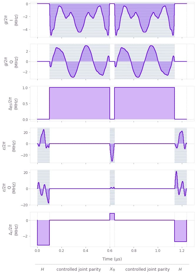
The above figure shows the full optimized pulse sequence. We now evaluate the infidelity of this pulse sequence for the cavities and the transmon ancilla which, in the closed system, can be attributed to coherent errors.
print(
    f"Infidelity of the full gate sequence: {result_rx['output']['infidelity_seq']['value']:.3e}"
)
Infidelity of the full gate sequence: 2.531e-05
One of the objectives of the optimization was to fulfill the "equal-latitude condition" during the gate sequence, that is, making the transmon latitude independent of the cavity state.
def plot_latitude(result_rx):
    plt.figure()
    sample_times = np.linspace(0, gate_duration_tot * 1e6, 7 * segment_count)
    latitude = result_rx["output"]["latitude_vz"]["value"]
    labels = [r"$|00\rangle$", r"$|01\rangle$", r"$|10\rangle$", r"$|11\rangle$"]

    for i, j in enumerate([0, 1, len(cardinal_states_c), len(cardinal_states_c) + 1]):
        plt.plot(sample_times, latitude[j] * 180 / np.pi, label=labels[i])

    plt.xlabel(r"Time ($\mu$s)")
    plt.ylabel("Latitude")
    plt.yticks(
        [0, 45, 90, 135, 180], [r"0", r"$\pi/4$", r"$\pi/2$", r"$3\pi/4$", r"$\pi$"]
    )
    plt.legend(title="Cavity states", bbox_to_anchor=(0.6, 0.48))
    plt.title("Transmon latitude for different initial cavity states")
    plt.show()


plot_latitude(result_rx)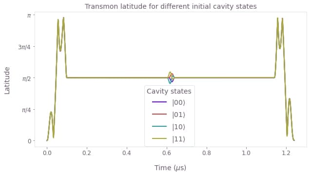
In the above plot, we see that the transmon latitude is independent of the cavity state for the majority of the protocol. Only during the $X_{\pi/2}$ gate on the transmon ancilla, we observe a slight deviation of the transmon latitude for different cavity states.
Optimization of noise robust pulses
We now take the susceptibility of the optimized pulses to errors in the control amplitudes as an exemplary noise source into account explicitly. To that end, we include quasi-static error terms in the Hamiltonian according to
\begin{align} g(t) &\rightarrow g(t) (1 + \delta g), \quad \epsilon(t) \rightarrow \epsilon(t) (1 + \delta \epsilon) \end{align}
with the relative amplitude errors $\delta g$ and $\delta \epsilon$ for the beamsplitter drive and the transmon drive, respectively.
with bo.cloud.group_requests():
    # First Hadamard gate.
    result_h_1_robust = optimize_hadamard(initial_state_t_h_1, robust=True)
    # Second Hadamard gate.
    result_h_2_robust = optimize_hadamard(initial_state_t_h_2, robust=True)
    # Ancilla-controlled joint parity gate.
    result_c_parity_robust = optimize_c_parity(robust=True)
    # RX gate.

print("Optimized first Hadamard gate.")
print(f"Cost: {result_h_1_robust['cost']:.3e}")
print(f"Gate infidelity: {result_h_1_robust['output']['infidelity']['value']:.3e}\n")

print("Optimized second Hadamard gate.")
print(f"Cost: {result_h_2_robust['cost']:.3e}")
print(f"Gate infidelity: {result_h_2_robust['output']['infidelity']['value']:.3e}\n")

print("Optimized ancilla-controlled joint parity gate.")
print(f"Cost: {result_c_parity_robust['cost']:.3e}")
print(
    f"Gate infidelity: {result_c_parity_robust['output']['infidelity']['value']:.3e}\n"
)

result_rx_robust = optimize_rx(
    result_h_1_robust, result_h_2_robust, result_c_parity_robust, robust=True
)
print("Optimized RX gate.")
print(f"Cost: {result_rx_robust['cost']:.3e}")
print(f"Gate infidelity: {result_rx_robust['output']['infidelity_rx']['value']:.3e}")
Optimized first Hadamard gate.
Cost: 2.016e-04
Gate infidelity: 7.527e-05
Optimized second Hadamard gate.
Cost: 2.156e-04
Gate infidelity: 1.097e-04
Optimized ancilla-controlled joint parity gate.
Cost: 3.344e-04
Gate infidelity: 3.342e-04
Optimized RX gate.
Cost: 2.543e-03
Gate infidelity: 8.004e-05
plot_pulse_sequence(result_rx_robust)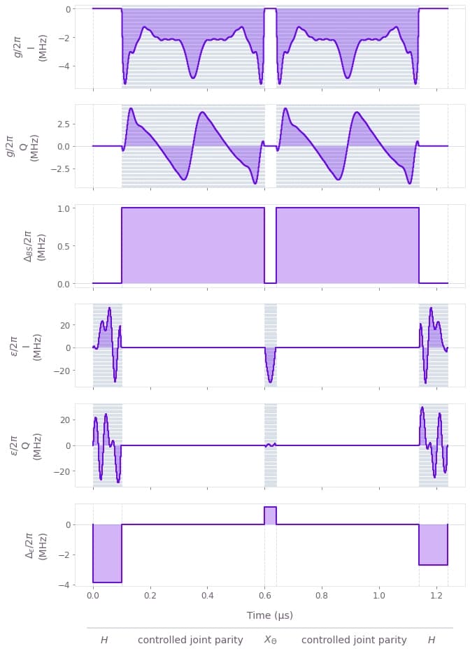
Looking at the optimized pulse sequence shown in the figure above, we see that especially for the Hadamard gates and the controlled joint parity gates, the robust pulses become more complex than the pulses obtained without the robustness criterion.
plot_latitude(result_rx_robust)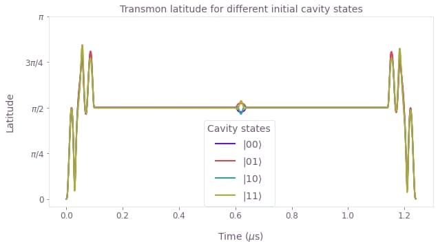
Also the transmon latitude shows a more complex behavior during the Hadamard gates than for the default optimization. Nevertheless, only during the $X_{\pi/2}$ gate, the latitude differs noticeably for different initial cavity states.
To investigate the robustness of the pulses, we perform a quasi-static scan over the amplitude errors and evaluate the infidelity for the $ZZ_{\pi/2}$ gate on the cavities and the gate failure probability, that is, the probability to measure the transmon in a different state than the ground state at the end of the protocol. We furthermore evaluate the impact of an additional detuning, treated as a quasi-static coherent error according to
\begin{align} \Delta_\text{BS}(t) &\rightarrow \Delta_\text{BS}(t) + \delta \Delta_\text{BS}, \quad \Delta_\epsilon(t) \rightarrow \Delta_\epsilon(t) + \delta \Delta_\epsilon. \end{align}
Here, we assume the same relative amplitude error and the same absolute detuning error for both the beamsplitter and the transmon drive.
def simulate_with_control_errors(result_rx, amplitude_error, detuning_error=0):
    graph = bo.Graph()

    # Optimized pulses.
    drive_c = graph.pwc(**result_rx["output"]["drive_c_seq"])
    delta_c = graph.pwc(**result_rx["output"]["delta_c_seq"])
    drive_t = graph.pwc(**result_rx["output"]["drive_t_seq"])
    delta_t = graph.pwc(**result_rx["output"]["delta_t_seq"])

    # Setup of the Hamiltonian.
    a, n_a, b, n_b, t, n_t, t_z, _, n_t_e = create_system_operators(
        graph, cavity_dim, transmon_dim
    )
    h_drift = (
        -chi / 2 * n_a @ t_z
        - k_a / 2 * (n_a @ n_a - n_a)
        - k_b / 2 * (n_b @ n_b - n_b)
        + chi_f_prime * (n_a @ n_a - n_a) @ n_t
        + chi_e_prime * (n_a @ n_a - n_a) @ (n_t_e - 2 * n_t)
        + chi_ab * n_a @ n_b
    )
    h_drive = (
        graph.hermitian_part(drive_c * (1 + amplitude_error) * graph.adjoint(a) @ b)
        + (delta_c + detuning_error) * n_a
        + graph.hermitian_part(drive_t * (1 + amplitude_error) * graph.adjoint(t))
        + (delta_t + detuning_error) * n_t
    )
    hamiltonian = h_drift + h_drive

    # Initial states of the gate sequence.
    initial_states_c = graph.reshape(
        graph.kronecker_product_list(
            [
                np.array(cardinal_states_c)[:, None, :, None],
                np.array(cardinal_states_c)[None, :, :, None],
            ]
        ),
        (len(cardinal_states_c) ** 2, cavity_dim * cavity_dim, 1),
    )
    target_states_c = (rzz @ initial_states_c)[:, :, 0]
    initial_state_t = np.array([1, 0, 0])
    initial_states = graph.reshape(
        graph.kronecker_product_list(
            [
                np.array(cardinal_states_c)[:, None, :, None],
                np.array(cardinal_states_c)[None, :, :, None],
                initial_state_t[:, None],
            ]
        ),
        (len(cardinal_states_c) ** 2, 1, cavity_dim * cavity_dim * transmon_dim, 1),
    )

    # Time evolution of the gate sequence.
    sample_times = np.linspace(0, gate_duration_tot, 7 * segment_count)
    unitaries = graph.time_evolution_operators_pwc(
        hamiltonian=hamiltonian, sample_times=sample_times
    )[None]
    evolved_states = (unitaries @ initial_states)[..., 0]

    # Infidelity of the target states and the evolved states of the gate sequence for the cavity subspace.
    states_c = graph.partial_trace(
        density_matrix=graph.outer_product(evolved_states, evolved_states),
        subsystem_dimensions=[cavity_dim, cavity_dim, transmon_dim],
        traced_subsystems=[2],
    )
    fidelity_c = graph.expectation_value(
        state=target_states_c, operator=states_c[:, -1]
    )
    infidelity_c = graph.sum(1 - graph.abs(fidelity_c)) / len(cardinal_states_c) ** 2
    infidelity_c.name = "infidelity_c"

    # Calculation of the transmon states during the gate sequence.
    states_t = graph.partial_trace(
        density_matrix=graph.outer_product(evolved_states, evolved_states),
        subsystem_dimensions=[cavity_dim, cavity_dim, transmon_dim],
        traced_subsystems=[0, 1],
    )

    # Gate failure probability.
    failure_probability = (
        graph.sum(graph.abs(states_t[:, -1, 1, 1]) + graph.abs(states_t[:, -1, 2, 2]))
        / len(cardinal_states_c) ** 2
    )
    failure_probability.name = "failure_probability"

    return bo.execute_graph(
        graph=graph, output_node_names=["infidelity_c", "failure_probability"]
    )


# Relative amplitude errors we scan over.
sample_count_evaluation = 55
amplitude_errors_evaluation = np.linspace(-0.1, 0.1, num=sample_count_evaluation)
detuning_error = 20 * 1e3

results = {
    "Optimal, no detuning": [],
    "Robust, no detuning": [],
    "Optimal, detuning": [],
    "Robust, detuning": [],
}

with bo.cloud.group_requests():
    for amplitude_error in amplitude_errors_evaluation:
        results["Optimal, no detuning"].append(
            simulate_with_control_errors(result_rx, amplitude_error)
        )
        results["Robust, no detuning"].append(
            simulate_with_control_errors(result_rx_robust, amplitude_error)
        )
        results["Optimal, detuning"].append(
            simulate_with_control_errors(result_rx, amplitude_error, detuning_error)
        )
        results["Robust, detuning"].append(
            simulate_with_control_errors(
                result_rx_robust, amplitude_error, detuning_error
            )
        )

results_values = [
    [
        [result["output"][measure]["value"] for result in res]
        for measure in ["infidelity_c", "failure_probability"]
    ]
    for res in results.values()
]

fig, axs = plt.subplots(2, 2, figsize=(12, 8))
fig.suptitle(f"Quasi-static amplitude error scan", y=0.96)
ylabels = ["Gate infidelity", "Gate failure probability"]
bbox_dict = {"facecolor": "white", "edgecolor": "lightgrey", "alpha": 0.8}
titles = ["No detuning", "Detuning 20 kHz"]

for i in range(2):
    for j in range(2):
        axs[j][i].plot(
            amplitude_errors_evaluation, results_values[j * 2 + 1][i], label="robust"
        )
        axs[j][i].plot(
            amplitude_errors_evaluation,
            results_values[j * 2][i],
            label="optimal,\nnon-robust",
        )
        axs[j][i].legend()
        axs[j][i].set_title(titles[j])
        axs[j][i].set_xticks(np.linspace(-0.1, 0.1, num=5))
        axs[j][i].set_yscale("log")
        axs[j][i].set_ylabel(ylabels[i])
    axs[1][i].set_xlabel("Relative amplitude error")

fig.tight_layout()
fig.subplots_adjust(wspace=0.3, hspace=0.2)
plt.show()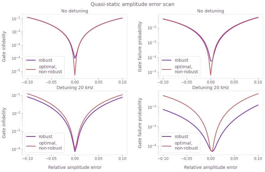
The robust pulse sequence outperforms the optimal, non-robust sequence and yields a lower infidelity for the $ZZ_{\pi/2}$ gate on the cavities as well as a lower gate failure probability already for small relative errors of the control amplitudes. With an additional detuning error, even without an amplitude error, the robust pulse sequence yields a lower infidelity than the optimal, non-robust sequence. Therefore, the robust pulse sequence is the better choice when an exact control amplitude and perfect pulse tuning cannot be guaranteed.
Open system validation
To assess the performance of the optimized pulse protocols under realistic conditions including incoherent noise, we simulate the $ZZ_{\pi/2}$ gate in an open system. Here, we focus on the decay and the dephasing of the transmon ancilla as well as the cavity decay while neglecting cavity dephasing which typically plays a minor role. Note that in the dual-rail construction, photon loss from the cavities can be detected separately via joint-parity measurements on the cavities forming a logical qubit so that it does not compromise the functioning of the error-detectable gate.
def simulate_open_system(
    result_rx, gamma_t=10000, gamma_phi_t=10000, cavity_decay=False, gamma_c=1000
):
    graph = bo.Graph()

    # Optimized pulses.
    drive_c = graph.pwc(**result_rx["output"]["drive_c_seq"])
    delta_c = graph.pwc(**result_rx["output"]["delta_c_seq"])
    drive_t = graph.pwc(**result_rx["output"]["drive_t_seq"])
    delta_t = graph.pwc(**result_rx["output"]["delta_t_seq"])

    # Setup of the Hamiltonian.
    a, n_a, b, n_b, t, n_t, t_z, t_e, n_t_e = create_system_operators(
        graph, cavity_dim, transmon_dim
    )
    h_drift = (
        -chi / 2 * n_a @ t_z
        - k_a / 2 * (n_a @ n_a - n_a)
        - k_b / 2 * (n_b @ n_b - n_b)
        + chi_f_prime * (n_a @ n_a - n_a) @ n_t
        + chi_e_prime * (n_a @ n_a - n_a) @ (n_t_e - 2 * n_t)
        + chi_ab * n_a @ n_b
    )
    h_drive = (
        graph.hermitian_part(drive_c * graph.adjoint(a) @ b)
        + delta_c * n_a
        + graph.hermitian_part(drive_t * graph.adjoint(t))
        + delta_t * n_t
    )
    hamiltonian = h_drive + h_drift

    # Decay terms.
    lindblad_terms = [(gamma_t, t_e), (gamma_phi_t, n_t_e)]
    if cavity_decay:
        lindblad_terms.append((gamma_c, a))
        lindblad_terms.append((gamma_c, b))

    # Initial and target states.
    initial_state_t = np.array([1, 0, 0])
    initial_states = graph.reshape(
        graph.kronecker_product_list(
            [
                np.array(cardinal_states_c)[:, None, :, None],
                np.array(cardinal_states_c)[None, :, :, None],
                initial_state_t[:, None],
            ]
        ),
        (len(cardinal_states_c) ** 2, -1, 1),
    )
    target_states = (rzz_tot @ initial_states)[..., 0]
    initial_dm = graph.outer_product(initial_states[..., 0], initial_states[..., 0])

    # Time evolution.
    sample_times = np.linspace(0, gate_duration_tot, 7 * segment_count)
    propagated_states = graph.density_matrix_evolution_pwc(
        initial_density_matrix=initial_dm,
        hamiltonian=hamiltonian,
        lindblad_terms=lindblad_terms,
        sample_times=sample_times,
    )

    # Evolved transmon states.
    states_t = graph.partial_trace(
        density_matrix=propagated_states,
        subsystem_dimensions=[cavity_dim, cavity_dim, transmon_dim],
        traced_subsystems=[0, 1],
    )

    # Calculate the error-detected infidelity.
    projector_g = graph.embed_operators(
        (np.array([[1, 0, 0], [0, 0, 0], [0, 0, 0]]), 2),
        [cavity_dim, cavity_dim, transmon_dim],
    )
    p_g = graph.trace(projector_g @ propagated_states[:, -1])
    projected_states = (projector_g @ propagated_states[:, -1] @ projector_g) / p_g[
        :, None, None
    ]
    fidelity_detected = graph.expectation_value(
        state=target_states, operator=projected_states
    )
    infidelity_detected = (
        graph.sum(1 - graph.abs(fidelity_detected)) / len(cardinal_states_c) ** 2
    )
    infidelity_detected.name = "infidelity_detected"

    # Gate failure probability.
    failure_probability = (
        graph.sum(graph.abs(states_t[:, -1, 1, 1]) + graph.abs(states_t[:, -1, 2, 2]))
        / len(cardinal_states_c) ** 2
    )
    failure_probability.name = "failure_probability"

    return bo.execute_graph(
        graph=graph, output_node_names=["infidelity_detected", "failure_probability"]
    )


# Simulation without noise.
result_simulation_default = simulate_open_system(
    result_rx, gamma_t=1e-6, gamma_phi_t=1e-6
)
result_simulation_robust = simulate_open_system(
    result_rx_robust, gamma_t=1e-6, gamma_phi_t=1e-6
)
print(f"Without noise:")
print(
    f"Error-detected infidelity: {result_simulation_default['output']['infidelity_detected']['value']:.3e},",
    f"gate failure probability: {result_simulation_default['output']['failure_probability']['value']:.3e} (optimal, non-robust)",
)
print(
    f"Error-detected infidelity: {result_simulation_robust['output']['infidelity_detected']['value']:.3e},",
    f"gate failure probability: {result_simulation_robust['output']['failure_probability']['value']:.3e} (robust)\n",
)

# Simulation with transmon decay and dephasing.
result_simulation_default = simulate_open_system(result_rx)
result_simulation_robust = simulate_open_system(result_rx_robust)
print("Transmon decay at T_1 = 100 us and transmon dephasing at T_phi = 100 us:")
print(
    f"Error-detected infidelity: {result_simulation_default['output']['infidelity_detected']['value']:.3e},",
    f"gate failure probability: {result_simulation_default['output']['failure_probability']['value']:.3e} (optimal, non-robust)",
)
print(
    f"Error-detected infidelity: {result_simulation_robust['output']['infidelity_detected']['value']:.3e},",
    f"gate failure probability: {result_simulation_robust['output']['failure_probability']['value']:.3e} (robust)\n",
)

# Simulation with additional cavity decay.
print("Additional cavity decay at T_1 = 1 ms:")
result_simulation_default = simulate_open_system(result_rx, cavity_decay=True)
result_simulation_robust = simulate_open_system(result_rx_robust, cavity_decay=True)
print(
    f"Gate failure probability: {result_simulation_default['output']['failure_probability']['value']:.3e} (optimal, non-robust)"
)
print(
    f"Gate failure probability: {result_simulation_robust['output']['failure_probability']['value']:.3e} (robust)"
)
Without noise:
Error-detected infidelity: 8.558e-07, gate failure probability: 2.445e-05 (optimal, non-robust)
Error-detected infidelity: 6.436e-06, gate failure probability: 2.970e-05 (robust)
Transmon decay at T_1 = 100 us and transmon dephasing at T_phi = 100 us:
Error-detected infidelity: 5.345e-05, gate failure probability: 2.321e-02 (optimal, non-robust)
Error-detected infidelity: 6.132e-05, gate failure probability: 2.373e-02 (robust)
Additional cavity decay at T_1 = 1 ms:
Gate failure probability: 2.374e-02 (optimal, non-robust)
Gate failure probability: 2.425e-02 (robust)
We observe that the gate failure probability increases significantly when considering an open system. However, the interesting measure for the open system is the error-detected infidelity, that is, the infidelity of the gate when measuring the transmon in the ground state at the end of the protocol. The error-detected infidelity remains at a very low level even in the presence of decoherence, indicating a very low level of second-order errors that evade detection.
Compared to the results Tsunoda et al. obtain employing a GRAPE-based pulse optimization, without noise, the pulses optimized using Boulder Opal give about 26x lower $ZZ_\Theta$ gate infidelity (about 3x for the robust sequence) and about 300x lower gate failure probability (about 24x for the robust sequence). Also in the presence of noise, taking into account a noisy ancilla with a decay time of $T_1 = 100 \mu\text{s}$ and a dephasing time of $T_\phi = 100 \mu\text{s}$, Boulder Opal yields an about 3x lower error-detected infidelity and a slightly lower gate failure probability which is also the case with additional cavity decay. Note that we furthermore included higher-order corrections to the Hamiltonian in our optimizations and simulations which are generally regarded as an obstacle to high-fidelity gates.
use_saved_results = True

gamma_count = 11
gamma_values = np.logspace(3, 5, gamma_count)

if use_saved_results:
    file_name = "resources/open_system_parameter_sweep"
    with open(file_name, "r+") as file:
        res = jsonpickle.decode(file.read())
        results_default = res[0]
        results_robust = res[1]

else:
    results_default = []
    results_robust = []
    with bo.cloud.group_requests():
        for gamma in gamma_values:
            for gamma_phi in gamma_values:
                results_default.append(
                    simulate_open_system(
                        result_rx, gamma_t=gamma, gamma_phi_t=gamma_phi
                    )
                )
                results_robust.append(
                    simulate_open_system(
                        result_rx_robust, gamma_t=gamma, gamma_phi_t=gamma_phi
                    )
                )
def gather_values(results, name):
values = [
results[gamma_count * i + j]["output"][name]["value"]
for i in range(gamma_count)
for j in range(gamma_count)
]
return np.reshape(values, (gamma_count, gamma_count))
plot_data = {
"Error-detected infidelity, default": gather_values(
results_default, "infidelity_detected"
),
"Error-detected infidelity, robust": gather_values(
results_robust, "infidelity_detected"
),
"Gate failure probability, default": gather_values(
results_default, "failure_probability"
),
"Gate failure probability, robust": gather_values(
results_robust, "failure_probability"
),
}
fig, axs = plt.subplots(2, 2, figsize=(10, 10))
fig.subplots_adjust(wspace=0.4, hspace=0.4)
norms = [
LogNorm(vmax=plot_data["Error-detected infidelity, default"].max()),
LogNorm(vmax=plot_data["Gate failure probability, default"].max()),
]
cmap = qv.QCTRL_SEQUENTIAL_COLORMAP.reversed()
for ax, title, norm in zip(
axs.flatten(), plot_data, [x for pair in zip(norms, norms) for x in pair]
):
cax = ax.pcolor(gamma_values, gamma_values, plot_data[title], norm=norm, cmap=cmap)
plt.colorbar(cax, ax=ax)
ax.set_title(title)
ax.set_xscale("log")
ax.set_yscale("log")
ax.set_xlabel(r"$\gamma$ (Hz)")
ax.set_ylabel(r"$\gamma\_\phi$ (Hz)")
plt.show()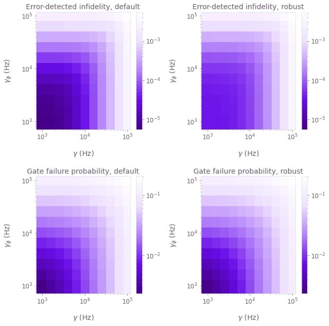
Evaluating the error-detected gate infidelity and the gate failure probability for a broad range of ancilla decay rates $\gamma$ and dephasing rates $\gamma_\phi$, we verify the robustness of our optimized pulses against incoherent noise. While the default pulse sequence performs slightly better for very low levels of noise under the assumption of no control amplitude errors, the performance does not differ significantly for higher noise levels. Overall, the error-detected infidelity remains well below 0.01% for a range of decay and dephasing rates that is realistic in current hardware, taking advantage of the gate design in combination with high-quality pulses optimized using Boulder Opal.