Boost signal-to-noise by 10X in cold-atom sensors using robust control
Using Boulder Opal robust Raman pulses to boost fringe contrast in tight-SWAP cold atom interferometers by an order of magnitude
Boulder Opal provides a flexible and comprehensive set of optimization tools capable of delivering augmented hardware performance to applications from quantum computing through to quantum sensing. Cold atom interferometers provide state-of-the-art gravitational and magnetic field sensitivity under laboratory conditions. However, when deployed in the field, their performance is limited by a combination of challenges arising from the laser instabilities, such as power, frequency, and phase fluctuations. We show how this issue can be addressed by designing control solutions for cold atom interferometers optimized for robustness against two simultaneous noise mechanisms:
- Laser intensity fluctuations often encountered in the field by processes such as fiber coupling jitter and thermal expansion of the atom cloud,
- The detuning processes, such as thermal momentum distribution of the atoms or the fluctuations in the laser frequency and phase.
In this application note we will present a complete workflow—from optimization of control pulses under strong noise through to time-domain simulation of the interferometer performance. We will cover:
- Noise-robust control optimization for beam-splitter (BS) and mirror (M) pulses
- Control performance validation by calculating 2D quasi-static error-susceptibility
- Time-domain end-to-end simulation of the interferometer to compare primitive and robust controls.
Ultimately we demonstrate how under high noise conditions, the Boulder Opal robust pulses increase the fringe contrast by an order of magnitude compared to primitive square pulses used in conventional settings.
Imports and initialization
import time
import jsonpickle
import numpy as np
import matplotlib as mpl
import matplotlib.pyplot as plt

from qctrlopencontrols import new_primitive_control
import qctrlvisualizer as qv
import boulderopal as bo

plt.style.use(qv.get_qctrl_style())

# Physical constants.
h_bar = 1.054571817e-34
c_light = 3e8
k_b = 1.380649e-23

# Rb atom parameters.
m_Rb = 86.9092 * 1.6605e-27
lamda = 780 * 1e-9  # m
k_avr = 2 * np.pi / lamda


# Three-level matrices for the Raman Hamiltonian.
identity3 = np.eye(3)
sigma_m13 = np.array([[0, 0, 0], [0, 0, 0], [1, 0, 0]])
sigma_m23 = np.array([[0, 0, 0], [0, 0, 0], [0, 1, 0]])

# Driving parameters.
omega_eff = 2 * np.pi * 4.0 * 10e3  # Hz

# Detuning parameters.
small_delta = 0  # two-photon
big_delta = 10e9  # one-photon

# Dicts used to hold controls for M and BS pulses.
pi_half_pulse_controls = {}
pi_pulse_controls = {}

# Flag to load longer optimization and simulation results from files.
use_saved_data = True

# Files to save to or load from.
data_dir = "./resources/"
optimized_bs_pulse_file = data_dir + "AtomSensing_Optimized_BS_pulse"
optimized_m_pulse_file = data_dir + "AtomSensing_Optimized_M_pulse"
fringe_signals_file = data_dir + "AtomSensing_Fringe_signals"


# Helper functions.
def run_optimization(duration, target_operator):
    """
    Specify the control drive variables and cost function for the optimizer,
    and output optimization result.
    """
    number_of_segments = 256  # number of pulse segments
    number_of_optimization_variables = 128
    omega_max = omega_eff / np.sqrt(2)  # maximum effective Rabi rate
    cutoff_frequency = 4 * omega_eff
    shift_max = 5 * omega_eff  # p/m limit on the freq. shift control

    # Define parameters of the stochastic optimization.
    sample_count = 300

    # Create optimization graph.
    graph = bo.Graph()

    # Sample random variables from probability distribution.
    relative_deltas = graph.random.normal(
        mean=0, standard_deviation=1.0, shape=(sample_count,)
    )
    betas = graph.random.normal(mean=0, standard_deviation=0.4, shape=(sample_count,))

    # Set up for drive controls.
    I_signal = graph.filter_and_resample_pwc(
        pwc=graph.real_optimizable_pwc_signal(
            segment_count=number_of_optimization_variables,
            duration=duration,
            maximum=omega_max,
            minimum=-omega_max,
        ),
        kernel=graph.sinc_convolution_kernel(cutoff_frequency),
        segment_count=number_of_segments,
    )
    Q_signal = graph.filter_and_resample_pwc(
        pwc=graph.real_optimizable_pwc_signal(
            segment_count=number_of_optimization_variables,
            duration=duration,
            maximum=omega_max,
            minimum=-omega_max,
        ),
        kernel=graph.sinc_convolution_kernel(cutoff_frequency),
        segment_count=number_of_segments,
    )

    # Set up drive signal for export.
    drive_signal = I_signal + 1j * Q_signal
    drive_signal.name = "$\\omega$"

    # Set up for shift controls.
    S_signal = graph.filter_and_resample_pwc(
        pwc=graph.real_optimizable_pwc_signal(
            segment_count=number_of_optimization_variables,
            duration=duration,
            maximum=shift_max,
            minimum=-shift_max,
        ),
        kernel=graph.sinc_convolution_kernel(cutoff_frequency),
        segment_count=number_of_segments,
        name="$\\zeta$",
    )

    # Set up multiple quasi-static Hamiltonian terms.

    # Shift term (constant for all points).
    shift_term = S_signal * graph.pauli_matrix("Z") / 2.0

    # Create a batch of delta terms.
    delta_term = graph.constant_pwc_operator(
        duration=duration,
        operator=relative_deltas[:, None, None]
        * (-h_bar * k_avr**2 / m_Rb)
        * graph.pauli_matrix("Z")
        / 2.0,
    )

    # Create Hamiltonian drive terms.
    I_term = I_signal * graph.pauli_matrix("X") / 2.0
    Q_term = Q_signal * graph.pauli_matrix("Y") / 2.0

    # Combine into net drive term (with a batch of noises).
    beta_pwc = graph.constant_pwc(
        constant=betas, duration=duration, batch_dimension_count=1
    )
    drive_term = (1 + beta_pwc) * (I_term + Q_term)

    # Total batch of Hamiltonians.
    quasi_static_Hamiltonian = drive_term + shift_term + delta_term

    # Calculate sum of infidelities for all noise realizations.
    infidelity_batch = graph.infidelity_pwc(
        hamiltonian=quasi_static_Hamiltonian, target=graph.target(target_operator)
    )
    cost = graph.sum(infidelity_batch, name="cost")

    # Run optimization.
    return bo.run_stochastic_optimization(
        graph=graph,
        cost_node_name="cost",
        output_node_names=["$\\omega$", "$\\zeta$"],
        iteration_count=10000,
    )


def three_level_controls_from_open_pulse(pulse):
    """
    Map Open Controls pulses designed for a two-level system
    onto the three-level Raman Hamiltonian,
    achieving equivalent evolution of the two ground states.
    """
    # Move from effective Rabi rate to two equal laser drives rates.
    omega_1 = np.sqrt(pulse.rabi_rates / 2 * big_delta)
    omega_2 = pulse.rabi_rates / 2 * big_delta / omega_1

    # Assign half the effective phase to each drive.
    phasors_1 = omega_1 * np.exp(0.5j * pulse.azimuthal_angles)
    phasors_2 = omega_2 * np.exp(-0.5j * pulse.azimuthal_angles)

    controls = {
        "duration": np.sum(pulse.durations),
        "Omega_1": {"durations": pulse.durations, "values": phasors_1},
        "Omega_2": {"durations": pulse.durations, "values": phasors_2},
    }

    return controls


def three_level_controls_from_two_level_optimized_result(optimized_result):
    """
    Convert controls for the effective two-level system
    to the three-level Raman system.
    """
    controls = {}

    if "$\\omega$" in optimized_result:
        durations = optimized_result["$\\omega$"]["durations"]
        effective_phasors = optimized_result["$\\omega$"]["values"]

        omega_1 = np.sqrt(np.abs(effective_phasors) / 2 * big_delta)
        omega_2 = np.abs(effective_phasors) / 2 * big_delta / omega_1

        phases = np.angle(effective_phasors)
        phasors_1 = omega_1 * np.exp(-1j * phases / 2)
        phasors_2 = omega_2 * np.exp(+1j * phases / 2)

        controls["duration"] = np.sum(durations)
        controls["Omega_1"] = {"durations": durations, "values": phasors_1}
        controls["Omega_2"] = {"durations": durations, "values": phasors_2}

    if "$\\zeta$" in optimized_result:
        controls["zeta"] = optimized_result["$\\zeta$"]

    return controls


def calculate_unitary(controls, phase, beta, big_delta, small_delta):
    """
    Calculate the unitary evolution operator in the Raman system
    from a set of pulse controls, and system parameters.

    The input parameters (phase offset, amplitude noise beta, and
    momentum/detuning noises small_delta/big_delta) can be either
    scalars or (compatibly-shaped) batches. In that case, a batch
    of unitaries is returned, one for each input parameter set.
    """

    graph = bo.Graph()

    phase = np.array(phase)

    hamiltonian = 0.0

    if "Omega_1" in controls:
        values = (
            (1 + beta[..., None])
            * graph.exp(1j * phase[..., None] / 2)
            * controls["Omega_1"]["values"]
        )
        hamiltonian += 2.0 * graph.hermitian_part(
            graph.pwc(
                values=values,
                durations=controls["Omega_1"]["durations"],
                time_dimension=-1,
            )
            * sigma_m13
        )

    if "Omega_2" in controls:
        values = (
            (1 + beta[..., None])
            * graph.exp(-1j * phase[..., None] / 2)
            * controls["Omega_2"]["values"]
        )
        hamiltonian += 2.0 * graph.hermitian_part(
            graph.pwc(
                values=values,
                durations=controls["Omega_2"]["durations"],
                time_dimension=-1,
            )
            * sigma_m23
        )

    if "zeta" in controls:
        hamiltonian += graph.pwc(
            values=controls["zeta"]["values"], durations=controls["zeta"]["durations"]
        ) * (np.diag([-1.0, 1.0, 0.0]) / 2.0)

    drift = graph.constant_pwc(
        constant=big_delta[..., None, None] * np.diag([-1, -1, 0])
        + small_delta[..., None, None] * np.diag([0, -1, 0]),
        duration=controls["duration"],
        batch_dimension_count=len(beta.shape),
    )

    hamiltonian += drift

    unitaries = graph.time_evolution_operators_pwc(
        hamiltonian=hamiltonian,
        sample_times=np.array([controls["duration"]]),
        name="unitaries",
    )

    result = bo.execute_graph(graph, "unitaries")

    return result["output"]["unitaries"]["value"]


def calculate_infidelities(controls, phase, beta, big_delta, small_delta, target):
    """
    Calculate the infidelity with respect to some target operator
    of the evolution of a the Raman system, from a set of controls
    and system parameters.

    The input parameters (phase offset, amplitude noise beta, and
    momentum/detuning noises small_delta/big_delta) can be either
    scalars or (compatibly-shaped) batches. In that case, a batch
    of infidelities is returned, one for each input parameter set.
    """

    unitaries = calculate_unitary(
        controls=controls,
        phase=phase,
        beta=beta,
        big_delta=big_delta,
        small_delta=small_delta,
    )

    trace = lambda mat: np.trace(mat, axis1=-1, axis2=-2)
    herm = lambda mat: np.conj(np.transpose(mat))

    target_op = np.matmul(target, np.diag([1, 1, 0]))
    overlap = trace(herm(target_op) @ unitaries) / trace(herm(target_op) @ target_op)
    infidelity = (1 - np.abs(overlap) ** 2).squeeze()

    return infidelity


def pulse_1D_quasi_static_scan(controls, target, betas, del_pz_coefficients):
    """
    Performs a quasi-static scan against pairs of
    beta and del_pz_coefficient.

    betas and del_pz_coefficients need to be arrays of the same length.
    """

    big_deltas = np.array(big_delta + del_pz_coefficients * k_avr / m_Rb)
    small_deltas = np.array(-2 * del_pz_coefficients * k_avr / m_Rb)
    betas = np.array(betas)

    return calculate_infidelities(
        controls=controls,
        phase=0.0,
        beta=betas,
        big_delta=big_deltas,
        small_delta=small_deltas,
        target=target,
    )


def pulse_2D_quasi_static_scan(controls, target, betas, del_pz_coefficients):
    """
    Computes a 2D quasi-static scan for each combination of
    betas and del_pz_coefficients.
    """

    pz_axis, beta_axis = np.meshgrid(del_pz_coefficients, betas)

    big_deltas = np.array(big_delta + pz_axis * k_avr / m_Rb)
    small_deltas = np.array(-2 * pz_axis * k_avr / m_Rb)

    infidelities = calculate_infidelities(
        controls=controls,
        phase=0.0,
        beta=beta_axis,
        big_delta=big_deltas,
        small_delta=small_deltas,
        target=target,
    )

    return pz_axis, beta_axis, infidelities


# Read and write helper functions, type independent.
def save_variable(file_name, var):
    """
    Save a single variable to a file using jsonpickle.
    """
    with open(file_name, "w+") as file:
        file.write(jsonpickle.encode(var))


def load_variable(file_name):
    """
    Load a variable from a file encoded with jsonpickle.
    """
    with open(file_name, "r+") as file:
        return jsonpickle.decode(file.read())
Creating robust Boulder Opal pulses for atom interferometry
Here, we create the set of Raman pulses optimized to simultaneously suppress against two pathways in which physical noise channels feed into the Raman Hamiltonian, namely detuning and Rabi rate variations.
Interferometer model
Consider a three-level atomic system of mass $M$ with two hyperfine ground states $|1\rangle$ and $|2\rangle$ and a third excited state $|3\rangle$ with transition frequencies given by $\omega_{13}$ ($|1\rangle\leftrightarrow|3\rangle$), $\omega_{23}$ ($|2\rangle\leftrightarrow|3\rangle$), and $\omega_{12}$ ($|1\rangle\leftrightarrow|2\rangle$). The system is driven by two counterpropagating laser beams in the Raman configuration with frequencies $\omega_{1L}$ and $\omega_{2L}$, with wave vectors $k_{1L}$ and $k_{2L}$, respectively.
The corresponding system Hamiltonian for a single momentum family $p$ ($|1,p-\hbar k_{1L}\rangle$, $|2, p+\hbar k_{2L}\rangle$ and $|3, p\rangle$) is given as follows (see Moler, Weiss, Kasevich, and Chu):
\begin{align} H = \begin{pmatrix} -\Delta & 0 & \Omega_1\\ 0 & -(\Delta + \delta) & \Omega_2\\ \Omega_1^* & \Omega_2^* & 0 \end{pmatrix}, \end{align}
where $\Omega_1$ and $\Omega_2$ are the Rabi rates associated with $|1\rangle\leftrightarrow|3\rangle$ and $|2\rangle\leftrightarrow|3\rangle$ optical transitions, while $\Delta$ and $\delta$ are the one-photon and two-photon detunings:
\begin{align} \Delta &= \frac{p k_{1L}}{M} - \frac{\hbar k_{1L}^2}{2M} +\omega_{13} -\omega_{1L},\\ \delta &= -\frac{p(k_{1L}+k_{2L})}{M} + \frac{\hbar k_{1L}^2}{2M} -\frac{\hbar k_{2L}^2}{2M} -\omega_{12} +\omega_{1L}-\omega_{2L}. \end{align}
Now, define the average frequency $\omega$ and the average wavevector $k = \omega/c$ as constants, such that the frequency difference between the two laser beams is captured by the single control parameter $\zeta$:
\begin{align} \omega_{1L} & = \omega + \frac{\zeta}{2},\\ \omega_{2L} & = \omega - \frac{\zeta}{2}. \end{align}
In the regime of interest, the one-photon transitions are significantly detuned ($\Delta\gg|\Omega_1|,|\Omega_2|,\delta$), and we can adiabatically eliminate the excited state. Therefore, the effective two-level Hamiltonian for the two internal states $|1,p-\hbar k_{1L}\rangle$ and $|2 , p+\hbar k_{2L}\rangle$ becomes:
\begin{align} H_{\rm eff} = \frac{1}{2} \begin{pmatrix} \zeta & |\Omega_{\rm eff}|e^{i\phi}\\ |\Omega_{\rm eff}|e^{-i \phi} & - \zeta\\ \end{pmatrix}, \end{align}
where the $\Omega_{\rm eff}$ is effective Rabi rate an $\phi$ the relative phase between the laser beams:
\begin{align} &\Omega_{\rm eff} = \frac{\Omega_1\Omega_2^*}{2\Delta}, \\ &\phi = {\rm arg}(\Omega_1) - {\rm arg}(\Omega_2).\\ \end{align}
We focus on two noise channels: the thermal distribution of atomic momenta in the direction of the laser (z-axis), $\partial p_z$, and the fluctuations in the laser power characterized by the parameter $\beta$.
The momentum variations couple via the detuning terms, $\Delta\rightarrow \Delta + \frac{\partial p_z k}{2M}$ and $\delta\rightarrow \delta - \frac{\partial p_z k}{M}$, while the laser fluctuations couple multiplicatively via the Rabi rate as $\Omega_\text{eff}\rightarrow(1+\beta)\Omega_\text{eff}$, for $\beta\in [-1,\infty)$. Therefore, the effective two-level Hamiltonian is:
\begin{align} H_{\rm eff} = \frac{1}{2} \begin{pmatrix} \zeta -\frac{\partial p_z k}{M} & (1+\beta)|\Omega_{\rm eff}|e^{i\phi}\\ (1+\beta)|\Omega_{\rm eff}|e^{-i \phi} & - \zeta +\frac{\partial p_z k}{M} \\ \end{pmatrix}. \end{align}
The robust mirror and beam-splitter pulses
We use the effective two-level Hamiltonian to generate the robust control parameters $\Omega_{\rm eff}$, $\zeta$ and $\phi$ for the specified target operation, given pulse duration and the number of segments.
To optimize the pulses, we use Boulder Opal's stochastic optimization engine. We provide to it a batch of quasi-stastic noise values, randomly sampled at each step of the optimization from the probability distributions that are Gaussian, but whose standard deviations lie a little above those described in the section "Noise model" of this application note. Providing probability distributions whose noise values lie a little above the values of the noises of the actual system helps the optimizer to find more robust solutions.
The samples in these batches form a set of quasi-static noise "points" that pave an extensive region of the 2D noise space formed by the two noise channels: the laser amplitude fluctuations and thermal detuning. Each point describes the system's Hamiltonian that has been quasi-statically offset by a pair of noise terms ($\partial p_z$, $\beta$). The cost function is the sum of the control's infidelity across all points. Minimizing this cost function ensures that the control pulse performs its target operation with high fidelity when $\partial p_z$ and $\beta$ fall within the value of the standard deviation of the probability distribution. The approach is well suited to sensing applications in high amplitude-noise environments.
After we generate the robust beam-splitter and mirror pulses controls, we convert them to the full three-level Raman controls for analysis in further sections. Plotting of the control parameters is done via the Q-CTRL Visualizer Python package.
optimization_scheme = "Q-CTRL"

# Duration of one effective Rabi cycle period.
s = 2 * np.pi / omega_eff

# Beam-splitter pulse.
pi_half_duration = 8 * s
pi_half_target_operator = np.array(
    [[np.sqrt(2) / 2, -1j * np.sqrt(2) / 2], [-1j * np.sqrt(2) / 2, np.sqrt(2) / 2]]
)
if use_saved_data:
    results = load_variable(optimized_bs_pulse_file)
else:
    print("**Optimizing beam-splitter pulse**")
    start_time = time.time()
    results = run_optimization(pi_half_duration, pi_half_target_operator)
    save_variable(optimized_bs_pulse_file, results)
    print("run (in min):", (time.time() - start_time) / 60.0)


# Store results to the three-level controls dict.
pi_half_pulse_controls[optimization_scheme] = (
    three_level_controls_from_two_level_optimized_result(results["output"])
)

# Plot controls.
qv.plot_controls(results["output"])
plt.suptitle("Beam-splitter pulse", y=0.95)

# Mirror pulse.
pi_duration = 9 * s
pi_target_operator = np.array([[0.0, -1j], [-1j, 0.0]])
if use_saved_data:
    results = load_variable(optimized_m_pulse_file)
else:
    print("**Optimizing mirror pulse**")
    start_time = time.time()
    results = run_optimization(pi_duration, pi_target_operator)
    save_variable(optimized_m_pulse_file, results)
    print("run (in min):", (time.time() - start_time) / 60.0)

# Store results to the three-level controls dict.
pi_pulse_controls[optimization_scheme] = (
    three_level_controls_from_two_level_optimized_result(results["output"])
)

# Plot controls.
qv.plot_controls(results["output"])
plt.suptitle("Mirror pulse", y=0.95)
plt.show()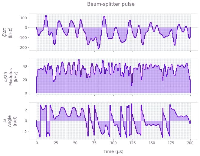
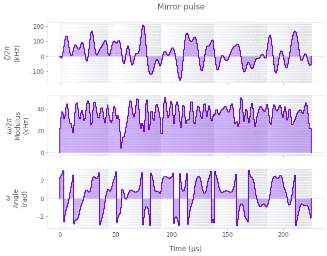
Plotted are the three control variables $\Omega_{\rm eff}$, $\phi$ and $\zeta$ as a function of time for the robust beam-splitter and mirror pulses. Note that the robust pulses can be built based on the specific selection of controls you use for your setup. For example, the control could only utilize a single parameter such as $\phi$ ($\Omega_{\rm eff}={\rm const}$, $\zeta=0$) or a combination of any two parameters. Filtering can be natively incorporated into the optimization process. For example, the pulses shown have a bandpass (sinc) filter with a cutoff of $4\Omega_{\rm eff}$.
Robustness verification with quasi-static scans
We can quantify the robustness of the control pulses by computing the infidelity of the three-level Raman unitary evolution as a function of the noise amplitude. The noise is treated in a quasi-static fashion over the duration of the pulse.
The performance of the robust pulses against the primitive square pulses will be compared for the following noise channels:
- The laser amplitude noise $\beta$,
- The atomic momentum deviation $\partial p_z$,
- The correlated combinations of noise from the two channels ($\partial p_z$,$\beta$).
We then benchmark the performance of the Boulder Opal robust pulses against the primitive square pulses most often used in cold atom interferometers. The square pulses are imported from Open Controls, and converted from the standard two-level format to the three-level Raman controls in order to form the beam-splitter ($\pi/2$) and mirror ($\pi$) pulses.
# Generate pulses from Open Controls and add to the list of pulse controls.
scheme = "primitive"

print(scheme, " mirror pulse created")
pi_pulse = new_primitive_control(
    rabi_rotation=np.pi, azimuthal_angle=0, maximum_rabi_rate=omega_eff
)
# Store the result in the control dict.
pi_pulse_controls[scheme] = three_level_controls_from_open_pulse(pi_pulse)

print(scheme, " beam-splitter pulse created")
pi_half_pulse = new_primitive_control(
    rabi_rotation=np.pi / 2, azimuthal_angle=0, maximum_rabi_rate=omega_eff
)
# Store the result in the control dict.
pi_half_pulse_controls[scheme] = three_level_controls_from_open_pulse(pi_half_pulse)
primitive mirror pulse created
primitive beam-splitter pulse created
Robustness to laser intensity fluctuations
Here the infidelity of the beam-splitter and mirror pulses is computed as a function of the laser fluctuation parameter $\beta$.
# Set the three-level unitary target operators for the BS and M pulses.
pi_half_target_operator = np.array(
    [
        [np.sqrt(2) / 2, 1j * np.sqrt(2) / 2, 0.0],
        [1j * np.sqrt(2) / 2, np.sqrt(2) / 2, 0.0],
        [0.0, 0.0, 1.0],
    ],
    dtype=complex,
)

pi_target_operator = np.array(
    [[0.0, 1j, 0.0], [1j, 0.0, 0.0], [0.0, 0.0, 1.0]], dtype=complex
)
# Quasi-static scan coefficients.
betas = np.linspace(-0.4, 0.4, 100)
del_pz_coefficients = np.zeros_like(betas)
# Pulse schemes
schemes = ["Q-CTRL", "primitive"]
colors = [qv.QCTRL_STYLE_COLORS[0], qv.QCTRL_STYLE_COLORS[1]]
fig, axs = plt.subplots(1, 2, figsize=(15, 5))
fig.suptitle("Robustness to fluctuations in laser amplitude", y=1.1)
# Quasi-static scan for BS pulse.
ax = axs[0]
ax.set_xlabel("$\\beta$")
ax.set_ylabel("Infidelity")
ax.set_title("Beam-splitter pulse")
ax.set_ylim(0, 0.7)
for idx, scheme in enumerate(schemes):
controls = pi_half_pulse_controls[scheme]
infidelities = pulse_1D_quasi_static_scan(
controls, pi_half_target_operator, betas, del_pz_coefficients
)
ax.plot(betas, infidelities, label=scheme, color=colors[idx])
# Quasi-static scan for M pulse.
ax = axs[1]
ax.set_xlabel("$\\beta$")
ax.set_ylabel("Infidelity")
ax.set_title("Mirror pulse")
ax.set_ylim(0, 0.7)
for idx, scheme in enumerate(schemes):
controls = pi_pulse_controls[scheme]
infidelities = pulse_1D_quasi_static_scan(
controls, pi_target_operator, betas, del_pz_coefficients
)
ax.plot(betas, infidelities, label=scheme, color=colors[idx])
hs, ls = axs[0].get_legend_handles_labels()
fig.legend(handles=hs, labels=ls, loc="center", bbox_to_anchor=(0.5, 1.0), ncol=2)
plt.show()Your task (action_id="1827918") is queued.
Your task (action_id="1827918") has completed.
Your task (action_id="1827919") has completed.
Your task (action_id="1827920") has started.
Your task (action_id="1827920") has completed.
Your task (action_id="1827921") has completed.
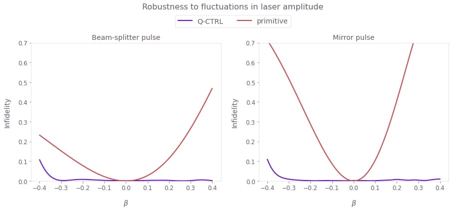
Depicted is the pulse infidelity as the function of the laser amplitude fluctuation $\beta$. Note that, in contrast to primitive square pulses, the infidelity of optimized pulses stays close to zero for an extensive range of laser power variations up to around $\pm30\%$. This is significant as the laser fluctuations of this magnitude are encountered, for example, in cloud expansion across the laser beams and impact of vibrations on fiber coupling in field-deployed interferometers.
Robustness to atom momentum variations
Next, compute the infidelity of the beam-splitter and mirror pulses as a function of the momentum variation of the atom $\partial p_z$.
del_pzs = (h_bar * k_avr) * np.linspace(-1.2, 1.2, 100)
betas = np.zeros_like(del_pzs)

fig, axs = plt.subplots(1, 2, figsize=(15, 5))
fig.suptitle("Robustness to variations in atom momentum", y=1.1)

# Quasi-static scan for BS pulse.
ax = axs[0]
ax.set_xlabel("$\\partial p\_z/(\\hbar k)$")
ax.set_ylabel("Infidelity")
ax.set_title("Beam-splitter pulse")
ax.set_ylim(0, 0.2)
for idx, scheme in enumerate(schemes):
    controls = pi_half_pulse_controls[scheme]
    infidelities = pulse_1D_quasi_static_scan(
        controls, pi_half_target_operator, betas, del_pzs
    )
    ax.plot(del_pzs / (h_bar * k_avr), infidelities, label=scheme, color=colors[idx])

# Quasi-static scan for M pulse.
ax = axs[1]
ax.set_xlabel("$\\partial p\_z/(\\hbar k)$")
ax.set_ylabel("Infidelity")
ax.set_title("Mirror pulse")
ax.set_ylim(0, 0.2)
for idx, scheme in enumerate(schemes):
    controls = pi_pulse_controls[scheme]
    infidelities = pulse_1D_quasi_static_scan(
        controls, pi_target_operator, betas, del_pzs
    )
    plt.plot(del_pzs / (h_bar * k_avr), infidelities, label=scheme, color=colors[idx])


hs, ls = axs[0].get_legend_handles_labels()
fig.legend(handles=hs, labels=ls, loc="center", bbox_to_anchor=(0.5, 1.0), ncol=2)

plt.show()
Your task (action_id="1827922") has completed.
Your task (action_id="1827923") is queued.
Your task (action_id="1827923") has completed.
Your task (action_id="1827926") has started.
Your task (action_id="1827926") has completed.
Your task (action_id="1827931") is queued.
Your task (action_id="1827931") has started.
Your task (action_id="1827931") has completed.
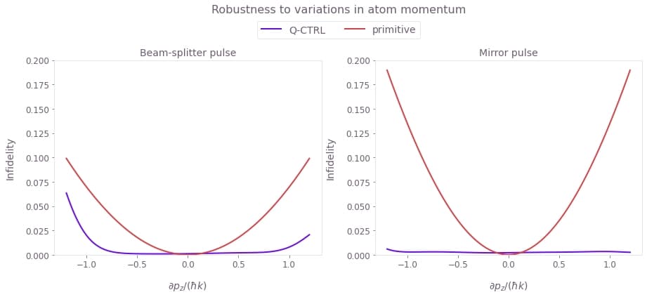
Plotted is the pulse infidelity as a function of deviation in the atom's momentum $\partial p_z$. Here, you can also see that, in contrast to primitive square pulses, the infidelity of optimized pulses stays flat for a wide range of momentum variations, up to around $\pm1k\hbar$. This is significant, as the given range overshoots typical experimental thermal spread in the atom clouds.
Robustness to noise in simultaneous channels
In the previous two sections, we focused on single-channel noise. However, the pulses are optimized to provide robustness against simultaneous noise channels. Using mirror pulses as an example, we test the performance of the pulses when both noise channels are present by plotting the infidelity on a 2D plane formed by the $\partial p_z$ and $\beta$ axes.
# Momentum noise coefficients.
del_pzs = h_bar * k_avr * np.linspace(-2, 2, 40)
# Laser noise coefficients.
betas = np.linspace(-0.6, 0.6, 40)

# Set up for 2D plot.
gs = mpl.gridspec.GridSpec(1, 2)
fig = plt.figure(figsize=(15, 5))
fig.suptitle(
    "Robustness correlated variations in atom momentum and laser amplitude", y=1
)

scheme = schemes[0]
for k, scheme in enumerate(schemes):
    # Quasi-static scan for the mirror pulses.
    (X, Y, Z) = pulse_2D_quasi_static_scan(
        pi_pulse_controls[scheme], pi_target_operator, betas, del_pzs
    )
    X = X / (h_bar * k_avr)

    # Plot 2D contours.
    ax = fig.add_subplot(gs[k])
    ax.set_title(scheme + " mirror pulse")
    ax.set_ylabel("$\\beta$")
    ax.set_xlabel("$\\partial p\_z/(\\hbar k)$")
    contours = ax.contour(X, Y, Z, levels=[0.01, 0.1], colors=qv.QCTRL_STYLE_COLORS[0])
    ax.clabel(contours, inline=True)

    plt.imshow(
        Z,
        extent=[np.min(X), np.max(X), np.min(Y), np.max(Y)],
        origin="lower",
        cmap=plt.colormaps["gray"].reversed(),
        alpha=0.8,
        aspect=np.abs((np.min(X) - np.max(X)) / (np.min(Y) - np.max(Y))),
        interpolation="bicubic",
        vmin=0,
        vmax=1,
    )
    cbar = plt.colorbar()
    cbar.set_label("Infidelity")

plt.show()
Your task (action_id="1827946") is queued.
Your task (action_id="1827946") has started.
Your task (action_id="1827946") has completed.
Your task (action_id="1827954") is queued.
Your task (action_id="1827954") has started.
Your task (action_id="1827954") has completed.
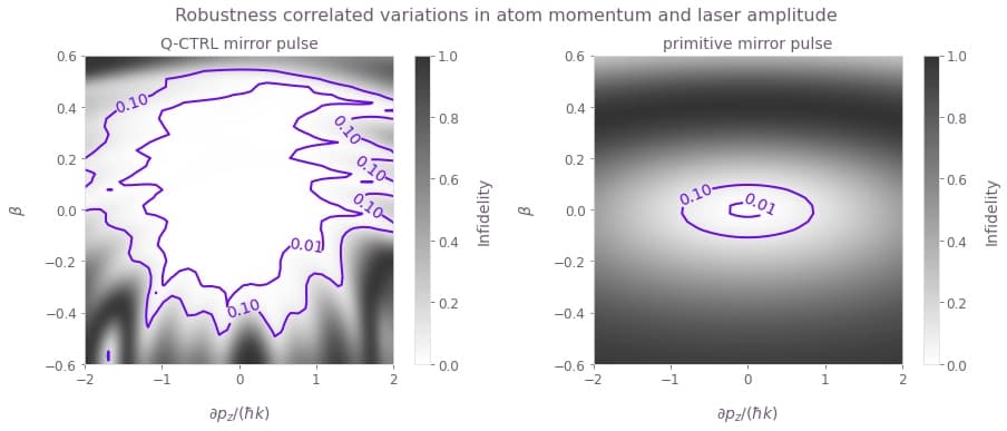
Plotted is the infidelity of the mirror pulse as a function of both $\partial p_z$ and $\beta$. To establish a relative comparison of the pulses' respective performance over the noise correlation space, observe that the area of the 0.01 infidelity contour of the robust pulses is around 30 times larger compared to the primitive square pulses. This is important experimentally because the atom's momentum and the laser amplitude variation form a highly correlated process during the thermal expansion of the atom cloud.
Improving interferometer fringe contrast with robust pulses
In order to demonstrate the impact of optimized pulses on atom interferometry, we simulate a Mach–Zehnder interferometer configuration for the atom cloud of typical thermal distribution under significant laser amplitude noise.
Noise model
The laser amplitude fluctuation process will be subject to a Gaussian distribution with the relatively broad standard deviation of $\sigma(\beta)=0.35$ reflective of the high noise environments. The thermal momentum noise process will have a standard deviation of $\sigma(\partial p_z) = 0.2\hbar k$, consistent with the thermal spread readily achievable in cold atom clouds.
ensemble_size = 2000  # number of noise processes samples

# Laser fluctuations, beta noise distribution.
beta_sigma = 0.35

# Set beta ensemble for each pulse.
beta_ensembles = {}
for scheme in schemes:
    beta_ensembles[scheme] = []
    for _ in ["BS", "M", "BS"]:
        betas_for_pulse = np.random.normal(0, beta_sigma, ensemble_size)
        betas_for_pulse = np.clip(betas_for_pulse, -1, None)
        beta_ensembles[scheme].append(betas_for_pulse)

# Thermal momentum noise.
del_pz_sigma = 0.2 * h_bar * k_avr  # momentum width
pz0 = np.random.normal(0, del_pz_sigma, ensemble_size)

# Compute ensemble of detunings.
small_deltas = -2 * pz0 * k_avr / m_Rb
big_deltas = big_delta + pz0 * k_avr / m_Rb
fig, axs = plt.subplots(1, 2, figsize=(15, 5))
fig.suptitle("High noise environment processes", y=1)
# Plot laser noise.
ax = axs[0]
ax.set_xlabel("$\\beta$")
ax.set_ylabel("Probability density")
ax.set_title("Laser pulse amplitude distribution")
count, bins, ignored = ax.hist(
beta_ensembles["primitive"][0], 30, density=True, color=qv.QCTRL_STYLE_COLORS[2]
)
amplitude_distribution = np.exp(-(bins**2) / (2 * beta_sigma**2)) / (
beta_sigma * np.sqrt(2 * np.pi)
)
ax.plot(bins, amplitude_distribution, "gray")
# Plot momentum distribution.
ax = axs[1]
ax.set_xlabel("$\\partial p\_z/(\\hbar k)$")
ax.set_ylabel("Probability density")
ax.set_title("Thermal momentum distribution")
count, bins, ignored = plt.hist(
pz0 / (h_bar * k_avr), 30, density=True, color=qv.QCTRL_STYLE_COLORS[1]
)
thermal_distribution = (h_bar * k_avr / del_pz_sigma / np.sqrt(2 * np.pi)) * np.exp(
-(bins**2) / (2 * (del_pz_sigma / (h_bar * k_avr)) ** 2)
)
plt.plot(bins, thermal_distribution, "gray")
plt.show()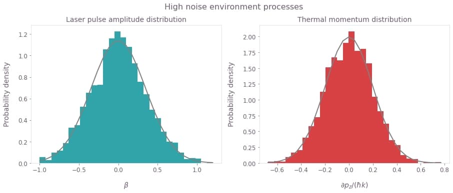
Depicted are the laser intensity and the atom cloud momentum distributions.
Simulation of full interferometric sequence
Here we simulate the total Mach–Zehnder interferometry sequence (BS-M-BS) and compare the primitive and the robust pulses. To do this we sample from the two outlined noise distributions to compute an ensemble of signals which is then averaged.
Laser amplitude fluctuations across the pulses in the Mach–Zehnder sequence are uncorrelated, reflecting relatively long flight time compared to the pulse duration. In contrast, the momentum noise is entirely correlated across the pulse sequence, reflecting low atom collision probability after the release of the cloud. The relative phase on the last beam-splitter pulse is varied in order to produce the fringe signal.
if use_saved_data:
    signal_data = load_variable(fringe_signals_file)
else:
    signal_data = {}
    # Phase offset on the last BS pulse.
    phase_offsets = np.linspace(0, 6 * np.pi, 50)
    # Initial state of the atom.
    initial_state = np.array([1, 0, 0])

    start_time = time.time()
    for idx, scheme in enumerate(schemes):
        # Evolve unitary though Mach–Zehnder sequence.
        U_total = identity3

        # First beam-splitter pulse.
        U_BS1 = calculate_unitary(
            pi_half_pulse_controls[scheme],
            0,
            beta=beta_ensembles[scheme][0],
            big_delta=big_deltas,
            small_delta=small_deltas,
        )

        # Mirror pulse.
        U_M = calculate_unitary(
            pi_pulse_controls[scheme],
            0,
            beta=beta_ensembles[scheme][1],
            big_delta=big_deltas,
            small_delta=small_deltas,
        )

        # Second beam-splitter pulse.
        U_BS2 = calculate_unitary(
            pi_half_pulse_controls[scheme],
            phase_offsets[:, None],
            beta=beta_ensembles[scheme][2][None, :],
            big_delta=big_deltas[None, :],
            small_delta=small_deltas[None, :],
        )

        # Total unitary.
        U_total = (U_BS1 @ U_M @ U_BS2).squeeze()

        # Final |0> state population.
        signal_ensemble = np.abs(U_total.dot(initial_state)[..., 0]) ** 2

        signal_data[scheme] = {
            "phase_offsets": phase_offsets,
            "signal_average": np.average(signal_ensemble, axis=1),
            "standard_error": np.std(signal_ensemble, axis=1) / np.sqrt(ensemble_size),
        }

    save_variable(fringe_signals_file, signal_data)
    end_time = time.time()

    print("run time: ", (end_time - start_time) / 60, "min")
# Plot the fringes.
fig, ax = plt.subplots(figsize=(15, 5))
fig.suptitle(
"Mach–Zehnder interferometer: fringe contrast comparison between primitive and optimized pulses"
)
plt.xlabel("Phase offset $\\phi/\\pi$")
plt.ylabel("Fringe signal")
for idx, scheme in enumerate(schemes):
x = signal_data[scheme]["phase_offsets"] / np.pi
y = signal_data[scheme]["signal_average"]
y_std = signal_data[scheme]["standard_error"]
color = qv.QCTRL_STYLE_COLORS[idx]
plt.plot(x, y, "-", color=color, label=scheme)
ax.fill_between(
x,
y - y_std,
y + y_std,
hatch="||",
facecolor="none",
edgecolor=color,
linewidth=0.0,
label=f"{scheme}$\\pm\\sigma$",
)
ax.set_xlim([0, 6])
ax.legend()
plt.show()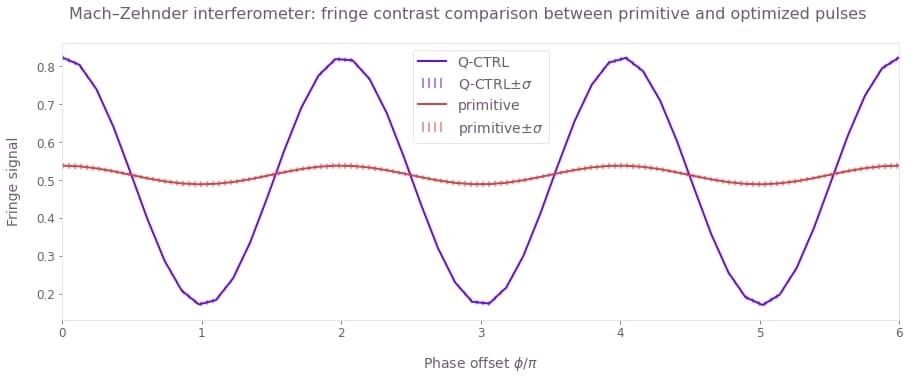
Plotted above is the average state probability $P_{|1\rangle}$ as a function of the phase offset on the last beam-splitter pulse. We see that operating the atom interferometer under high noise conditions using the standard square pulses causes the fringe contrast to suffer significantly under the noise distributions outlined above. In contrast, our robust pulses exhibit ten times greater fringe contrast.
