How to run custom variational algorithms
Running variational algorithms with the `iterate` function
Fire Opal's iterate function is optimized for submitting multiple jobs, which makes it an excellent tool for running variational quantum algorithms (VQAs). Compared to the execute function, which should be used for single-job submission, the iterate function optimizes preprocessing and device queuing time when jobs are submitted in immediate succession.
Variational quantum algorithms involve iteratively adjusting the parameters of a parameterized quantum circuit to optimize an objective function, ultimately finding approximate solutions to optimization problems or simulating quantum systems.
In this guide, you will learn how to use Fire Opal's iterate feature for variational quantum algorithms.
Summary workflow
The following steps describe the general workflow for running variational quantum algorithms.
1. Prepare the variational ansatz
Design a parameterized quantum circuit (PQC) that represents the problem. This circuit typically includes variational parameters that can be adjusted to minimize some cost function.
2. Define the objective function
Define a cost function that quantifies how well the quantum circuit solves the problem. This cost function typically depends on the outcomes of measurements performed on the quantum circuit.
3. Run the optimization loop using iterate
Initialize the parameters of the PQC and execute it on the quantum hardware. Calculate the cost function and use classical optimization methods to continuously adjust the parameters until reaching desired convergence criteria.
4. Evaluate results
Analyze the final solution obtained from the quantum circuit execution.
Example: Running the Variational Quantum Eigensolver (VQE) algorithm with iterate
In this example, the iterate function is used to run a sample 3-qubit VQE algorithm that obtains the lowest eigenvalue of the observable $\hat{O} = Z_0I_1X_2 - 0.5Z_0X_1I_2 + 0.5I_0X_1X_2$. This example is used as a demonstration, and the iterate function can easily be applied to other VQAs using similar patterns.
There are numerous tutorials available online that dive further into the theory and structure of building a VQE algorithm, such as this demonstration by Pennylane.
1. Import libraries and set up credentials
import fireopal as fo
from qiskit.circuit.library import TwoLocal
from qiskit import QuantumCircuit
from qiskit import qasm3
import numpy as np
from scipy.optimize import minimize
from fireopal.types import PauliOperator
In this example, the iterative workload is run on IBM Quantum. The following code builds a credentials object using credentials that can be obtained on the IBM Quantum Platform dashboard.
# Set credentials
token = "YOUR_IBM_CLOUD_API_KEY"
instance = "YOUR_IBM_CRN"

credentials = fo.credentials.make_credentials_for_ibm_cloud(
    token=token, instance=instance
)
2. Prepare the variational ansatz
This example uses parameterized quantum circuits, which are supported in both Fire Opal's iterate and execute functions. PQCs must be converted to OpenQASM 3.0 for submission to Fire Opal.
# Prepare the initial state, specifically flipping the states of qubits 0 and 2 to |1> using X-gates
initial_state = QuantumCircuit(3)
initial_state.x(0)
initial_state.x(2)
initial_state.barrier()

# Define the variational ansatz using the TwoLocal circuit template
qc = TwoLocal(
    num_qubits=3,
    rotation_blocks=["ry"],
    entanglement_blocks="cx",
    entanglement="full",
    initial_state=initial_state,
    reps=1,
    flatten=True,
    insert_barriers=True,
)
qc.barrier()

# Rotate qubits for a Z-basis measurement
# No rotation needed for qubit 0 as it aligns with Pauli Z
qc.h(1)  # Apply Hadamard gate to qubit 1 to measure in X basis
qc.h(2)  # Apply Hadamard gate to qubit 2 to measure in X basis

qc.measure_all()
qc.draw("mpl")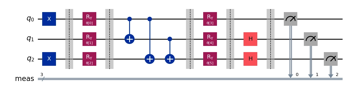
# Convert to OpenQASM3
qasm_circ = qasm3.dumps(qc)
3. Set initial parameters
# Set up initial parameters or default to zeros
init_params = np.zeros(len(qc.parameters))
4. Define the objective function
When performing iterative optimization, the cost function determines the objective to minimize. In VQE, the objective is to minimize the expectation value of the Hamiltonian to find the ground state energy of the quantum system. iterate is used to run the parameterized circuit with the updated parameters and return values used to compute the expectation value.
# Set shot count and define backend
# To get a list of supported backends, run fo.show_supported_devices(credentials)
shot_count = 2048
backend_name = "desired_backend"
# Store the history of calculated expectation values
expectation_value_history = []
def convert_probabilities_to_list(probabilities, nqubits):
"""
Transforms a dictionary of measured probabilities to a list of
probabilities in the computational basis.
"""
probs = []
for key in range(2**nqubits):
binary_key = format(key, "b").zfill(nqubits)
probs.append(probabilities.get(binary_key, 0))
return probs
def objective_function(parameters):
"""
Calculates the cost based on the quantum circuit's outcome.
Maps numerical parameters to the circuit parameters, runs the circuit, and computes the expectation value.
"""
# Map the parameters to the circuit parameters
parameters_dict = {param.name: val for param, val in zip(qc.parameters, parameters)}
observables = PauliOperator.from_list([("ZIX", 1), ("ZXI", -0.5), ("IXX", 0.5)])
job = fo.iterate_expectation(
circuits=[qasm_circ],
shot_count=shot_count,
credentials=credentials,
backend_name=backend_name,
parameters=[parameters_dict],
observables=observables,
)
expectation_value = job.result()["expectation_values"][0]
# Save the intermediate cost values without additional calls to this objective function
global expectation_value_history
expectation_value_history.append(expectation_value)
return expectation_value5. Run the optimization loop using iterate
You can choose a classical optimizer to minimize the cost function. In this case, the COBYLA solver from SciPy is applied through the minimize function. Once the minimize routine has completed, call stop_iterate to close the session on IBM Quantum systems in order to reduce total runtime.
# Set options to limit max iterations
options = {"maxiter": 30, "rhobeg": 0.5, "disp": True}

# Minimize the objective function using COBYLA method
opt_result = minimize(
    objective_function, init_params, method="COBYLA", tol=0.01, options=options
)

# Stop iterating once convergence is reached
fo.stop_iterate(credentials, backend_name)
6. Evaluate results
Once the algorithm has converged or reached the maximum number of iterations, you can evaluate the final expectation value and the history across each iteration. You can visually confirm that the expectation value decreases and converges to the ideal solution.
final_expectation_value = opt_result["fun"]
print("\n" f"Final value of the ground-state energy = {final_expectation_value}")
Final value of the ground-state energy = -1.384765625
import matplotlib.pyplot as plt

plt.figure(figsize=(10, 5))
plt.plot(
    expectation_value_history,
    marker="o",
    linestyle="-",
    color="#680CE9",
    label="Fire Opal",
)
plt.title("Expectation Value History Over Optimization Iterations")
plt.xlabel("Iteration")
plt.ylabel("Expectation Value")
plt.hlines(-2.0, 0, 30, linestyles="dashed", color="grey", label="Ideal solution")
plt.legend()
plt.show()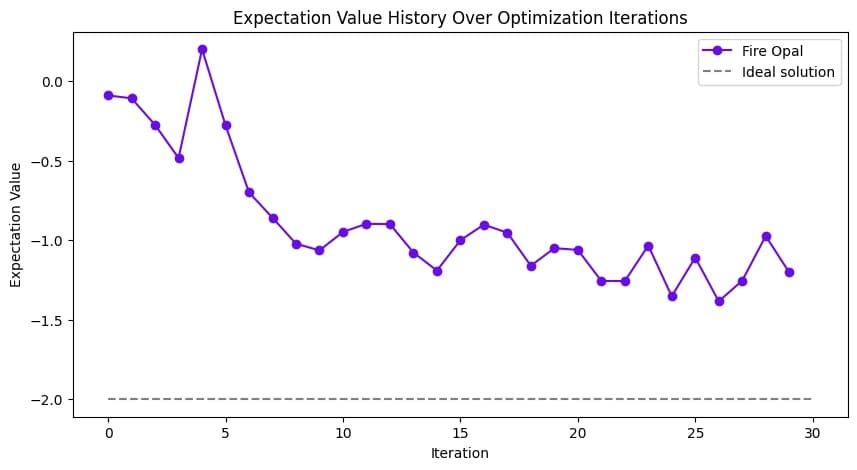
from fireopal import print_package_versions

print_package_versions()
| Package | Version |
| --------------------- | ------- |
| Python | 3.12.9 |
| matplotlib | 3.10.1 |
| networkx | 2.8.8 |
| numpy | 2.3.0 |
| qiskit | 1.4.2 |
| qiskit-ibm-runtime | 0.36.1 |
| sympy | 1.13.3 |
| fire-opal | 8.6.1 |
| qctrl-workflow-client | 5.5.1 |
